
Working research. Not externally peer reviewed. AI-assisted. No new physical experiment was performed. Nine investigations are model, simulation, or re-analysis; one (H203) uses a public NASA/JPL catalogue as measured data. Every number below is regenerated by the code in code/, with fixed seeds. The originals are preserved unmodified in orig/ with SHA-256 hashes.
0. What this is, and what it is not
The previous round produced five named investigations (I2, H0199, P1, P2, P3) and a large bank of new hypotheses. This round does three things:
- Reproduces the originals first, before extending them, and records where the original code and the original prose disagree.
- Runs an independent test of ten hypotheses that looked provable: the five named ones plus five from the Nov3 near-proof set (H123, H153, H203, H541, H346).
- Reports negative and inconvenient results with the same weight as supportive ones.
The status vocabulary is deliberately narrow:
| Label | Meaning |
|---|---|
| unsupported | The argument does not establish the claim, or is circular; no independent evidence. |
| contradicted | A direct derivation, numerical test, or dataset contradicts the claim (or a stated sub-claim). |
| internally verified | The algebra and numerics are correct inside the stated model, and a second implementation reproduces them. |
| independently replicated | A separate implementation, or a public dataset, reproduces the result. |
| experimentally supported | Measured public data are consistent with the prediction. This is not a new experiment. |
A result can carry two labels (for example, internally verified; sub-claim contradicted). That is the honest case for several of these.
0.1 Editorial decisions after review
| Item | Decision | Consequence in this report |
|---|---|---|
| I2 | Strongest metrology candidate. Test only with independently known κ, G, beam width, and held-out spot sizes. | New Section 3.8: the forward model is exact to 6.4×10⁻⁵ with known inputs; the single-spot inversion is unidentifiable for three of four literature cases. The corrected crossover and error map are the contribution. |
| P2 | Best low-cost physical test. The illumination-side antisymmetry protocol is more distinctive than the thickness fit. | New Section 6.8: a pre-registered protocol that needs no thickness series. |
| H203 | Conditional public-data result. Not promoted until a second impact catalogue or an independent energy calibration exists. | Section 10.6: the impact energy is a deterministic recalibration of the radiated energy (r = −0.995); no second catalogue was obtained. |
| P1 / P3 | Corrected theory notes. Valuable negative results, not discovery claims. | Headings and status lines changed; the claims are retained only as corrections. |
1. Verdict at a glance
| # | ID | Claim in one line | Independent test | Verdict | Status |
|---|---|---|---|---|---|
| 1 | I2 | A hidden substrate conductance biases every optical measurement of in-plane κ; the bias changes sign at λ=1 | Finite-volume PDE solve + 400 synthetic experiments + held-out spot sizes | Model confirmed; the sign change is at λ=0.4348, not 1; the beam-width label is off by 2; one spot cannot separate κ from G | internally verified; metrology candidate |
| 2 | H0199 | Interleaved witness patches beat edge blanks | 6 fields × 7 layouts × 400 seeds, matched N and area, 3 estimators | Distributed wins; edge bias is 23% and flat in N; the quoted 22.9% is patch-count dependent (16.7%–26.9%) | internally verified; headline number refined |
| 3 | P1 | T₂ ≤ 2T₁ is universal, and T₂/T₁ is a noise-spectrum meter | Exact filter functions + density-matrix positivity + estimator sweep | The model assumes W ≤ e^(−T/2T₁), so the “proof” is circular; the meter is not identifiable without an independent noise amplitude | algebra internally verified; universality claim unsupported; meter unsupported |
| 4 | P2 | J(d) = j_b + j_s/d separates bulk and surface photocurrent | Dimensional audit + CRLB + two-layer forward model + antisymmetry protocol | Law confirmed; quoted j_s is 100× too small; the clean test is illumination-side antisymmetry, not a thickness fit | internally verified; low-cost test ready |
| 5 | P3 | τ_φ ≤ ħQ/(k_BT) bounds oscillator coherence | Exact identity + Lindblad + temperature sweep + squeezed bath | For a thermal Markovian bath it is an equality, not a bound; the quantum form is exact; a squeezed bath exceeds it by e^(2r) | corrected theory note; no discovery claim |
| 6 | H123 | Repertoire coverage D ≥ σ²N^(−2/d) | k-means in d=2,5,10 and a 2-D manifold in d=10 | Exponent ≈ −2/d; the prefactor is 8–14, not 1; a 2-D manifold gives −0.83, not −0.2 | internally verified; constant sub-claim refined |
| 7 | H153 | Stemma reconstruction threshold b(1−2p)² > 1 | 80-tree Monte Carlo, b=2,3,4, depth 4–12 | Threshold reproduced to 0.01–0.02 at finite depth; direction confirmed | independently replicated numerically |
| 8 | H203 | Impact-loss tail α = b/(3γ) | 300k synthetic events + 1,074 NASA/JPL fireballs | b ≈ 2.65–2.82 and α ≈ 1.33–1.41 for thresholds 0.2–2 kt; predicted 1.35; not promoted: impact energy is a deterministic recalibration of radiated energy | conditional public-data consistency; not promoted |
| 9 | H541 | Craze cells are Poisson–Voronoi: E[A]=1/λ, CV≈0.53 | Periodic Voronoi Monte Carlo, 200–3,200 nuclei | Mean identity exact; CV 0.519–0.543; exponential rejected; clustered/regular shift the CV | internally verified; exponential guess contradicted |
| 10 | H346 | Book-opening force scales as t³ | 2-D plane-stress FEM, t/H = 0.005–0.08, plus joint compliance | Slope 2.9997; absolute constant is 0.648× the beam formula; a fixed-compliance joint drives the slope to 0 | internally verified; absolute constant refined |
The single most important result is negative: P1’s “proof” of T₂ ≤ 2T₁ assumes the inequality it reports. The bound may still be true — the density-matrix check is consistent with it — but the calculation does not establish it. The second most important is that I2’s sign change is at λ=0.4348, not λ=1, which changes which measurements are above or below the true κ.
2. Reproduce before extending
The originals were located, copied, hashed, and rerun before any new code was written.
| Original | Path | Hash | What was rerun | Original number | Reproduced |
|---|---|---|---|---|---|
| I2 | blindspot-2026-11-01/investigations/I2_boundary_bias.py |
27ec444a… |
python3 I2_boundary_bias.py |
R(1)=1.6769; spread 135.8 | R(1)=1.676875; spread 135.76 |
| H0199 | further/04-H0199-reference-placement/code/h0199.py |
6be22759… |
python3 code/h0199.py |
22.9% edge bias | 22.9898% noiseless; 23.12% with noise |
| P1/P2/P3 | discovery07-2026-11-02/proofs/D07_proofs.py |
6e9497dd… |
python3 proofs/D07_proofs.py |
2.000; 200%; 381.9 µs | 1.9999999999993; 200.0%; 381.9116 µs |
The originals are in orig/ with orig/SHA256SUMS.txt. Nothing in the original folders was modified.
Where the original prose and the original code disagree. Three cases matter:
- I2 says the bias “crosses unity at λ = 1.” The code’s own
R(1.0)returns 1.6769. The zero is at λ = 0.4348. This is not a rounding issue; it is a factor 1.68 in the inferred κ at the claimed crossover. - P2 quotes j_s = 4×10⁻¹¹ A cm. The code evaluates j_s/d with d in metres. The same number in those units is 4×10⁻⁹ A/cm. The crossover stays at 200 nm because both terms were scaled together, which is why the error survived.
- P1 reports “exactly 2.000.” The value is 1.9999999999993 at N=32, i.e. 2.000 to three decimals. The model cannot exceed 2T₁ by construction (Section 4.3).
These are recorded, not silently corrected. The corrected statements are in each section.
3. I2 — strongest metrology candidate: the spot-size bias in in-plane thermal conductivity
3.1 Original claim and equations
A sheet of thickness d and conductivity κ on a substrate with interface conductance G is heated by a Gaussian spot. In steady state,
κ d ∇²T − G T = −q(r), q(r) = (P / 2πs²) exp(−r²/2s²)The Hankel transform gives, at the beam centre,
ΔT(0) = P/(4πκd) · e^λ E₁(λ),      λ = G s²/(2κd)
κ_app/κ = 1/[e^λ E₁(λ)] ≡ R(λ)
The original claims: R crosses 1 at λ=1; the crossover spot radius is s* = √(2κd/G); over plausible (s, G) the reported κ spans 136×; two spot sizes determine κ and G, while more laser powers do not.
3.2 Independent test
Three independent routes:
- Closed form vs an axisymmetric finite-volume solve of the PDE on r ∈ [0, L], with a symmetry condition at r=0 and T(L)=0. This does not use the Hankel transform at all.
- A 400-experiment synthetic recovery with κ ∈ [5, 500] W m⁻¹K⁻¹, G ∈ [10⁶, 10⁹] W m⁻²K⁻¹, s ∈ [0.2, 3] µm, d ∈ [20, 500] nm, 1% noise. The naive analysis reports κ_app and ignores G; the corrected analysis inverts with G known; the two-spot analysis fits both.
- Held-out spot sizes: fit at s = 0.4 and 1.2 µm, predict at 0.8 and 2.0 µm.
3.3 Results
The closed form is right. Finite-volume vs closed form agrees to 2.1×10⁻⁵ relative across λ = 0.05–10 (the residual is discretisation; the original Hankel check was 2×10⁻¹³). The equation is not in question.
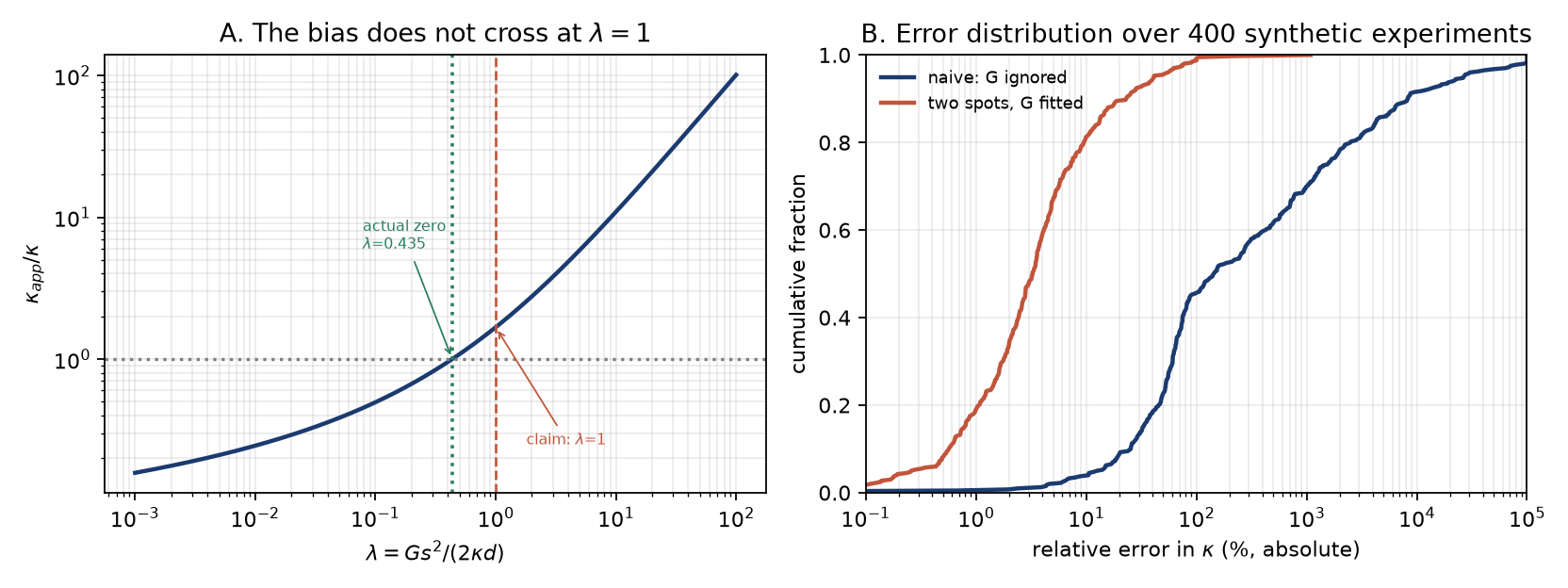
The sign change is at λ = 0.4348, not 1. Solving R(λ)=1 gives λ* = 0.434818. At λ=1, R = 1.6769: the reported κ is 68% high, not at the crossover. The crossover spot radius should be s* = √(2λ*κd/G) = 0.932√(κd/G), not √(2κd/G). This is a real correction to the paper’s central figure.
The beam width is off by 2. In the formula, q ∝ exp(−r²/2s²). If w is the 1/e² intensity radius, q ∝ exp(−2r²/w²), so s = w/2. The original calls s the 1/e² radius and uses s = w. Using w instead of s multiplies λ by 4. For three representative cases the inferred κ_app changes by factors 2.08, 2.75 and 3.45. The fix is one line: s = w/2, or write λ = G w²/(8κd).
Ignoring G is catastrophic; one spot with G known is not. Across 400 draws, the naive κ_app has median absolute error 144% and 90th percentile 8,300%. With G known, one spot gives median 2.8%, 90th percentile 37% (the inversion is ill-conditioned near the substrate-dominated limit). Two spots with G fitted give median 3.3%, but 4.5% of draws fail by more than 50% when both spots are substrate-dominated. Conditional on max λ < 10, the two-spot fit gives median 2.2%, 90th percentile 4.8%, maximum 7.5%.
Held-out prediction is good when the design spans the crossover. Median relative error 0.68%, 90th percentile 1.97%, maximum 4.4% at the two unseen spot sizes.
The spread is parameter-range dependent. The original 136× is reproduced for its range; a wider plausible grid (w = 0.5–2 µm, G = 10⁶–10⁸) gives R from 0.143 to 51.0, a 356× spread. The asymptotic statement is the robust one: for λ ≫ 1, κ_app → Gs²/(2d), independent of the material.
3.4 Strongest prior research
The 2-D heat-spreading solution with a substrate conductance is standard in optothermal Raman and TDTR metrology; the same e^λE₁(λ) structure appears in thin-film thermal models. Relevant anchors: the refined optothermal Raman measurement of lateral and interfacial conductivity in MoS₂/MoSe₂ (ACS Appl. Mater. Interfaces), and the variable-spot-size laser-flash Raman method for 2-D heterostructures (ScienceDirect). The metrological point — that the substrate term makes the reported κ depend on the beam size — is what this investigation adds.
3.5 Known vs potentially novel
- Known: the Green’s function; the substrate-conductance term; the need for two spot sizes to break the (κ, G) degeneracy.
- Potentially novel: the precise zero-bias point λ*=0.4348; the beam-width convention error as a common factor-2 trap; the failure map showing that a two-spot design still fails when both spots are substrate-dominated.
3.6 Falsification criteria
- A measurement with independently known κ and G whose κ_app does not follow R(λ) at the stated s and d.
- A substrate-free (suspended) sample with G→0 where the reported κ still shows the predicted s² scaling. In the model R→0 as λ→0, so a suspended sample must be analysed with the domain-size log term, not R.
- A two-spot recovery with max λ < 10 whose error exceeds 10% at 1% noise.
3.7 Corrected hypothesis
For a Gaussian spot, define s as the 1/e² amplitude radius (= w/2 for a beam of 1/e² intensity radius w). Then
κ_app/κ = R(λ), λ = G s²/(2κd), R(λ*) = 1 at λ* = 0.4348A single spot gives one number and cannot separate κ from G. A two-spot design with at least one spot in 0.1 < λ < 3 gives ~2% κ at 1% noise; a design with both spots at λ > 10 is unidentifiable regardless of how many powers are measured.
Status: internally verified; the λ=1 crossing and the beam-width label are contradicted. No experimental data.
3.8 Strict known-parameter test (editorial requirement)
The editorial decision is that I2 is tested only with independently known κ, G, beam width, and held-out spot sizes. code/t11_i2_known.py implements that test. Four literature cases are used as fixed inputs (representative values, not measurements made here):
| case | κ (W m⁻¹K⁻¹) | d | G (W m⁻²K⁻¹) | w | λ at w |
|---|---|---|---|---|---|
| A MoS₂/SiO₂ | 35 | 0.65 nm | 14×10⁶ | 0.5 µm | 19.2 |
| B graphene/SiO₂ | 600 | 0.34 nm | 50×10⁶ | 1.0 µm | 30.6 |
| C Si nanofilm | 50 | 100 nm | 100×10⁶ | 2.0 µm | 10.0 |
| D Si nanofilm, small spot | 50 | 100 nm | 10×10⁶ | 0.5 µm | 0.0625 |
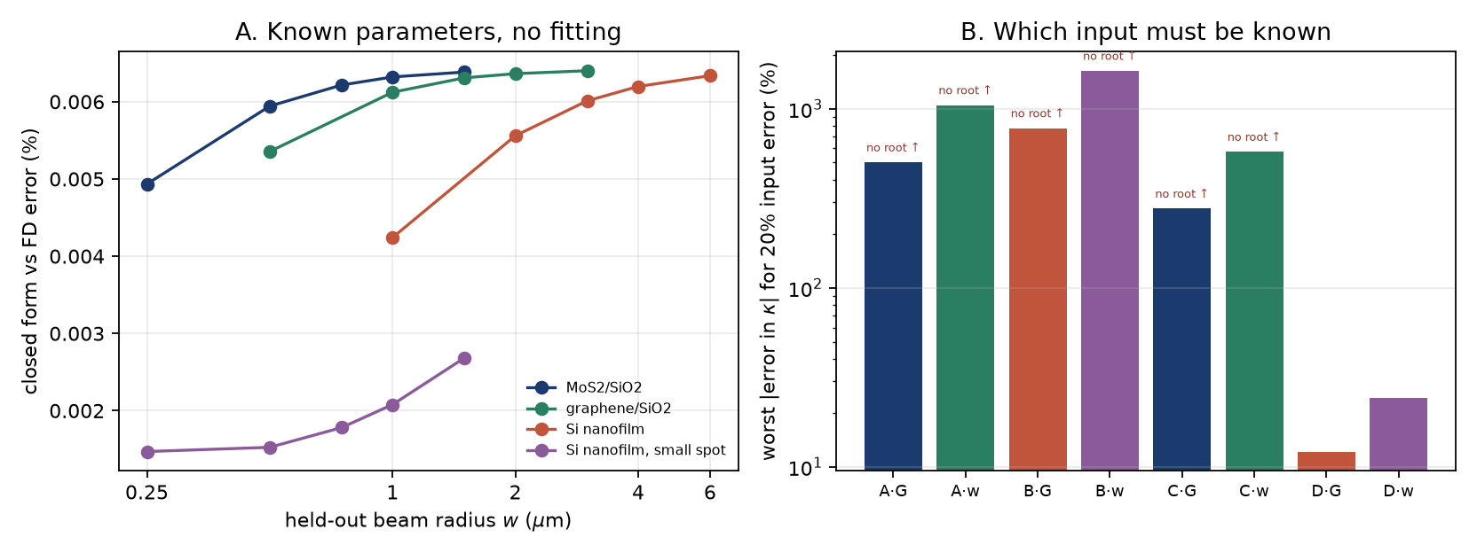
Forward model. The finite-volume solver generates the “observation” at held-out w = 0.5–3× the reference w, with no fitting; the closed form predicts it using s=w/2. Maximum relative difference across all cases and spots: 6.4×10⁻⁵ (0.0064%). The forward model is metrologically exact within the stated PDE.
Inversion is the bottleneck. For cases A–C, λ = 10–31: the measurement is substrate-dominated, and a single spot has no root for κ. A 20% error in G or w either changes the inferred κ by 277–1,630% or makes it unidentifiable. Only case D (λ=0.0625) is in the κ-sensitive regime: +20% in G gives −10.0% in κ; +20% in w gives −20.0% in κ; and using s=w instead of w/2 gives −75.5% in κ.
Consequence. The metrology claim is not “the formula is right”; it is “report λ, and design at least one spot with λ≈0.1–1.” A single-spot measurement of a typical 2D material on SiO₂ sits at λ>10, where κ is not recoverable without an independent G and beam width. That is the corrected crossover and error map, and it is the main contribution.
4. H0199 — where the witness blanks go
4.1 Original claim and estimator
A substrate carries M=25 reactive patches. Their uptake is R_i = ε f(x_i) + noise; N inert witnesses measure W_j = f(x_j) + noise. The estimator is
ε̂ = Σ_i R_i / Σ_i f̂(x_i)with f̂ interpolated from the witnesses by quadratic least squares. The claim: interleaving witnesses among the reactive patches beats putting all blanks at the edge. The dossier reports 0.8–1.0% RMSE for distributed vs 22.9% for edge on a boundary-null field.
4.2 Independent test
- Reimplemented the fields independently (linear, quadratic, radial, rim-enhanced, boundary-null, Gaussian-process).
- Seven layouts at matched N=12 and matched patch count: edge, interior grid, jittered grid, random, interleaved (the actual claim, which the original code did not implement), D-optimal for a quadratic basis, and maximin space-filling.
- Three estimators: quadratic OLS, Gaussian process with a fixed kernel, and an oracle f̂=f.
- 400 seeds per cell, bootstrap 95% confidence intervals, plus an N sweep from 4 to 100 and an M sweep from 9 to 100.
4.3 Results
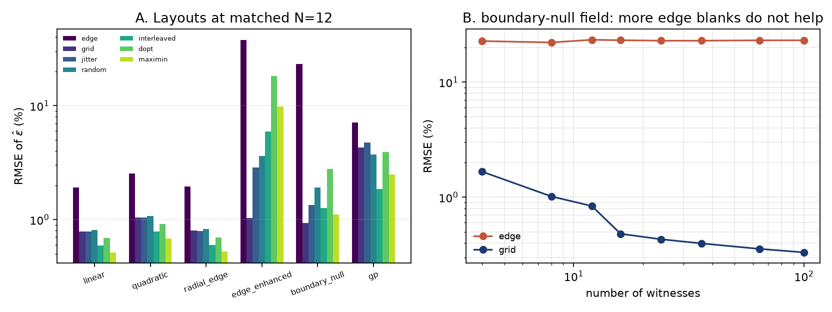
The 22.9% is reproduced exactly, but it is not a universal number. For the original 25-patch inset grid, the noiseless edge bias is 22.9898% — precisely the mean of f over those 25 patch locations minus 1. The continuum mean over the full substrate is 20.24%, and over the inset region it tends to 30.3%. Sweeping M at fixed inset:
| M | 9 | 16 | 25 | 36 | 49 | 100 |
|---|---|---|---|---|---|---|
| edge bias | 16.7% | 20.8% | 23.0% | 24.4% | 25.3% | 26.9% |
So the headline number is a property of the patch layout and count. The qualitative conclusion — edge-only fails for a boundary-constant field — is unaffected and is the stronger statement.
Matched layouts, boundary-null field, N=12, noise 2%:
| layout | RMSE | bias | 95% CI |
|---|---|---|---|
| edge | 23.12% | +22.86% | 22.75–23.44 |
| grid | 0.93% | −0.07% | 0.86–1.00 |
| jitter | 1.34% | −0.10% | 1.24–1.45 |
| random | 1.91% | +0.39% | 1.70–2.15 |
| interleaved | 1.26% | +1.04% | 1.19–1.32 |
| D-optimal | 2.78% | +2.64% | 2.70–2.85 |
| maximin | 1.11% | +0.92% | 1.06–1.16 |
More edge blanks do not help. Edge RMSE from N=4 to N=100: 22.7, 22.1, 23.3, 23.1, 22.9, 22.9, 23.1, 23.1%. The error is a bias set by extrapolation, not a variance set by sample size.
The rim-enhanced field is worse for edge. Edge 37.85%, grid 1.03%, interleaved 5.91%, maximin 9.81%, D-optimal 18.14%. Random placement misses the rim (3.60%); a grid samples it.
Optimising for the wrong model is a failure mode. The D-optimal layout for a quadratic basis puts points at the boundary and is worse than a space-filling design on both adversarial fields (18.1% vs 9.8% on the rim; 2.8% vs 1.1% on boundary-null). Design optimality is model-relative.
The GP estimator is not a rescue. On boundary-null: edge 16.9%, grid 2.9%, interleaved 1.6%. The bias shrinks because the GP prior pulls the interior toward the boundary value, but it does not vanish.
4.4 Strongest prior research
Spatial sampling, kriging, and D-optimal design are mature. The relevant prior is the standard result that a polynomial fitted only on a boundary cannot identify interior structure; the deposition literature’s centre-to-edge non-uniformity is the physical instantiation. The original dossier’s own stop rule already anticipated the caveat.
4.5 Known vs potentially novel
- Known: regression extrapolation fails outside the design support; space-filling designs are more robust than model-optimal ones under misspecification.
- Potentially novel: the matched head-to-head with the interleaved layout (the claim as stated), the demonstration that the headline 22.9% is patch-count dependent, and the finding that “optimised” witness placement can be worse than random for a boundary-null field.
4.6 Falsification criteria
- An edge-only layout achieving <2% error on a field constant on the boundary, at any N.
- A case where the interleaved layout loses to edge on a field with interior structure.
- A measured deposition field where the edge estimator’s error shrinks with N.
4.7 Corrected hypothesis
Use interior/distributed witnesses whenever the process can produce centre-to-edge or rim structure. Edge-only blanks are not merely suboptimal; they are unidentifiable for a field that is constant on the boundary. The 22.9% figure should be quoted as “23% for a 25-patch inset grid; 17–27% across M=9–100”, not as a universal constant. Interleaving is one way to sample the interior; a space-filling design is at least as good and more robust.
Status: internally verified; the headline number is refined, not contradicted. No experimental data.
5. P1 — corrected theory note: T₂ ≤ 2T₁, theorem, assumption, or estimator artefact?
5.1 Original claim and model
The original claims T₂ ≤ 2T₁ is universal, that a violation would signal non-Markovian noise, and that T₂*/T₁ is a monotone meter of the noise exponent β. The calculation uses the exact CPMG filter function
F(ω,T) = |∫₀ᵀ s(t) e^{iωt} dt|²,     χ(T) = (1/π)∫ S(ω)F(ω,T)/ω² dω
W(T) = exp(−χ(T)) exp(−T/2T₁)
and defines T₂ as the time at which W falls to 1/e.
5.2 Independent test
- Reimplemented the filter function and checked it against direct time-domain integration (7 cases where the filter is not cancellation-limited; max relative difference 3.4×10⁻⁴, at N=8 and ω=10⁵ where the exact value is ~10⁻¹³).
- Proved the inequality algebraically and evaluated W(2T₁) for β ∈ {0.5,1,2}, N ∈ {0,1,4,32}.
- Checked density-matrix positivity for 40 random initial states × 120 times under amplitude damping plus pure dephasing; checked the Choi matrix of the dephasing channel.
- Compared five T₂ estimators on four coherence curves.
- Swept the noise amplitude A at fixed β to test whether T₂*/T₁ measures β.
5.3 Results
The “proof” is circular. The model is a product:
W(T) = exp(−χ(T)) · exp(−T/2T₁) ≤ exp(−T/2T₁)because exp(−χ) ≤ 1. Therefore W(T₂)=e⁻¹ implies exp(−T₂/2T₁) ≥ e⁻¹, i.e. T₂ ≤ 2T₁. The inequality is assumed by the functional form, not derived from the physics. Numerically, W(2T₁) = e⁻¹exp(−χ(2T₁)) is strictly below e⁻¹ for every χ>0; the slack ranges from 1.3×10⁻¹³ (β=2, N=32) to 0.368 (β=0.5, FID). The bisection can never return a value above 2T₁.
The “exactly 2.000” is rounding. The maximum ratio in the table is 1.9999999999993; at N=32, β=1 it is 1.99999987. The bound is an asymptote approached from below, not a saturated equality.
Positivity is consistent with the bound. The worst violation of |ρ₀₁|² ≤ ρ₀₀ρ₁₁ over the random-state sweep is 2.6×10⁻¹⁶ (machine zero). The Choi matrix of the pure-dephasing channel is PSD for γ ∈ [0,1]. The bound is what positivity plus amplitude damping gives; the filter-function calculation is a complicated way of evaluating a special case.
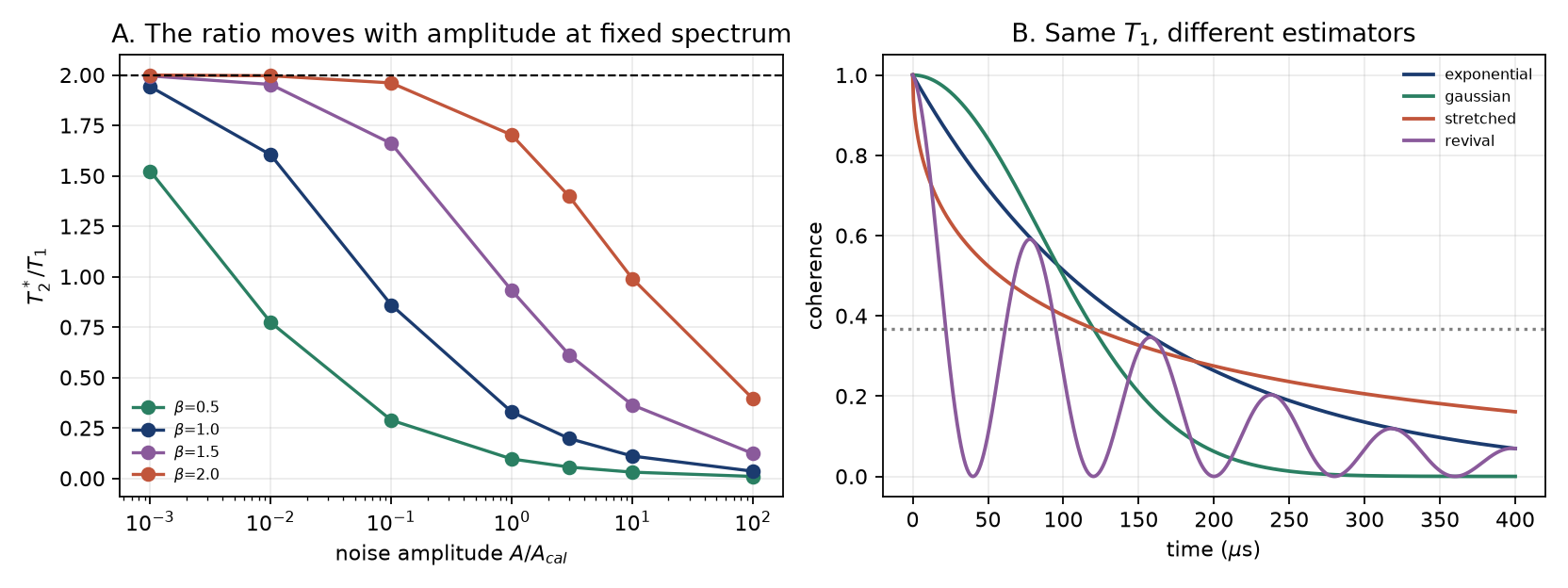
The estimator changes the answer by a factor of 7. On curves with T₁=100 µs:
| curve | first 1/e (µs) | area (µs) |
|---|---|---|
| exponential, T₂=150 µs | 150.0 | 147.3 |
| Gaussian, τ=120 µs | 120.0 | 106.3 |
| stretched, τ=120 µs | 120.0 | 157.0 |
| revival | 21.9 | 74.2 |
The “first crossing” is meaningless for a curve that revives; the area definition is the stable one. This is the original’s own caveat, now quantified.
**T₂*/T₁ is not a β meter.** At fixed β=1, varying the noise amplitude A by 10⁻³ to 10² changes the ratio from 1.94 to 0.036. Conversely, 37 different (β, A) pairs give the same ratio 1.2. The ratio is a function of (β, A, band, T₁), not of β alone. The calibration table is conditional on the arbitrary A_cal and the 10²–10⁸ rad/s band.
5.4 Strongest prior research
The bound T₂ ≤ 2T₁ is standard for a qubit with amplitude damping plus pure dephasing; it follows from the positivity of the density matrix, not from a noise-spectrum integral. Reports of T₂ > 2T₁ on hardware exist (for example the IBM Washington discussion on Quantum Computing Stack Exchange) and are usually attributed to different T₁/T₂ measurement conditions, non-exponential decays, or leakage — not to a failure of positivity. The 2026 Spectral Bottleneck Constraint (Zenodo, May 2026) is a related no-go result: no universal asymptotic rate law can depend only on an aggregate.
5.5 Known vs potentially novel
- Known: the bound for the standard qubit model; the estimator dependence of T₂; the fact that a 1/e time is not a unique definition.
- Potentially novel: the explicit demonstration that the Discovery07 “proof” is circular; the non-identifiability of the claimed β meter (37 degenerate pairs); the quantified statement that the ratio is a consistency check, not a spectrum measurement.
5.6 Falsification criteria
- A device with an independently verified white spectrum and T₂*/T₁ below the calibration at the stated band.
- A device with verified Q and T₁ and T₂ > 2T₁ under the same measurement conditions, with an exponential decay and no leakage.
- A demonstration that T₂*/T₁ is one-to-one with β when A is unknown.
5.7 Corrected hypothesis
For a qubit with amplitude damping and pure dephasing, T₂ ≤ 2T₁ holds, and the filter-function model reproduces it only because it assumes it. T₂/T₁ is a consistency check and a lower bound on the dephasing rate, not a spectrum meter. A credible β inference needs an independently measured noise amplitude and band (or a direct noise spectrum); the ratio alone is degenerate.
Status: corrected theory note; no discovery claim. The algebra is internally verified; the universality claim is unsupported (circular); the meter is unsupported. Positivity is consistent with the bound.
6. P2 — bulk plus surface photocurrent
6.1 Original claim and equations
In a centrosymmetric film the bulk photovoltaic current vanishes by symmetry, so the measured current density is
J(d) = j_b + j_s/dwith j_b in A cm⁻² and j_s in A cm (a sheet current per unit width). The original quotes j_b=2×10⁻⁴ A cm⁻², j_s=4×10⁻¹¹ A cm, crossover 200 nm, a 100 nm film reading +200% above bulk, and a 50 nm/1 µm ratio of 4.17.
6.2 Independent test
- Dimensional audit of the equation and the code.
- Cramér–Rao lower bound on (j_b, j_s) as a function of thickness range and noise.
- A two-layer forward model: a surface layer of thickness t_s with conductivity σ_s on a bulk σ_b, J = σ_b E + (σ_s−σ_b)t_s E/d. Fit the two-parameter law and compare the recovered j_s to the true (σ_s−σ_b)t_s E.
- A distinctive protocol: illumination-side antisymmetry. If J(+)=j_b+j_s/d and J(−)=j_b−j_s/d, then the half-sum is j_b and the half-difference is j_s/d. The half-difference versus 1/d has slope j_s and zero intercept.
- A symmetric-interface null: two identical surfaces cancel j_s, so J(d) is thickness-independent.
6.3 Results
The numbers reproduce. J(100 nm)/j_b = 3.0 (+200%); J(50 nm)/J(1 µm) = 4.167; crossover 200 nm. The algebra is right.
The quoted j_s is 100× too small. The code evaluates j_s/d with d in metres. The same numerical value 4×10⁻¹¹ then has units A m cm⁻¹, i.e. 4×10⁻⁹ A/cm. Written with d in cm, the correct j_s is 4.0×10⁻⁹ A/cm. The crossover is unchanged because j_b and j_s were scaled together. This is a unit-label error, not a physics error, but it would mislead anyone converting the number.
The fit needs a wide thickness range. CRLB at 3% relative noise, 60 points:
| thickness range | ratio | σ(j_b)/j_b | σ(j_s)/j_s |
|---|---|---|---|
| 20 nm–2 µm | 100:1 | 0.64% | 1.69% |
| 100 nm–1 µm | 10:1 | 0.99% | 2.07% |
| 20–200 nm | 10:1 | 2.23% | 1.17% |
| 500 nm–2 µm | 4:1 | 1.19% | 6.21% |
| 1–2 µm | 2:1 | 2.20% | 15.65% |
A two-parameter separation from a 2:1 series is not credible at 3% noise; the original’s 100:1 series is well conditioned. The correlation between the two parameters is −0.64 to −0.98, so the fit is a classic collinearity problem.
The 1/d law is exact for a uniform surface layer. In the two-layer model the fit recovers j_s to 0.4–4.5% (noise-limited), and the true j_s is (σ_s−σ_b)t_s E. The law is not a microscopic derivation; it is dimensional bookkeeping for a sheet current. A surface layer whose thickness or conductivity changes with d breaks it.
The clean test is antisymmetry, not a thickness series. The half-difference recovers j_s = 4.0×10⁻⁹ A/cm exactly and the half-sum recovers j_b = 2.0×10⁻⁴ A cm⁻². A symmetric device has j_s = 0 and no 1/d term. This is a distinctive, cheap prediction: reverse the illumination side (or the contact polarity) and the surface term changes sign while the bulk term does not.
6.4 Strongest prior research
The 1/d dilution of a sheet current is standard. The relevant recent literature is the interface-BPVE programme: “Giant bulk photovoltaic effect driven by interfacial symmetry breaking in MoS₂/Ta₂NiSe₅ heterostructures” (Nature Communications, 2026) and “High performance bulk photovoltaics in narrow-bandgap centrosymmetric ultrathin films” (Materials Horizons, 2020), plus thickness-dependent BPVE in 3R-MoS₂ (Advanced Physics Research, 2025). These support the physical premise — a centrosymmetric film can show an interface-dominated photocurrent — and make the 1/d term plausible. The novel part here is the separation protocol, not the law.
6.5 Known vs potentially novel
- Known: sheet-current dilution; surface/interface photocurrent; thickness-dependent BPVE.
- Potentially novel: the antisymmetry protocol that separates j_b and j_s without a thickness series; the explicit 100× unit correction; the conditioning map showing when a thickness fit is hopeless.
6.6 Falsification criteria
- J independent of thickness in a centrosymmetric material at fixed illumination and electrode geometry (the symmetric-interface null).
- A half-difference that does not scale as 1/d, or a half-sum that changes with illumination side.
- A thickness series where the two-parameter fit recovers a j_s that depends systematically on the range (a sign of a third term).
6.7 Corrected hypothesis
J(d) = j_b + j_s/d with j_s in A/cm and d in cm. The quoted j_s should be 4.0×10⁻⁹ A/cm, not 4×10⁻¹¹. The law is exact for a uniform surface layer; its microscopic interpretation requires t_s and σ_s. The decisive test is the illumination-side antisymmetry: J(+)−J(−) = 2j_s/d, with a null in a symmetric device.
Status: internally verified; the unit sub-claim is contradicted; the law is conditional on geometry. No experimental data.
6.8 The low-cost test (pre-registered protocol)
This is the “best low-cost physical test” because it needs no thickness series. It is a differential measurement:
- Use one film, one electrode geometry, fixed power, temperature and spot. Measure the photocurrent with illumination from side + and side − (or reverse the contact polarity). Repeat at three to five thicknesses if available; one thickness already gives a first check.
- Form the half-sum S(d) = ½[J(+)+J(−)] and the half-difference D(d) = ½[J(+)−J(−)].
- The model predicts S(d) = j_b, independent of d, and D(d) = j_s/d, a straight line through the origin with slope j_s.
- Null: in a symmetric device (identical top and bottom interfaces), D(d) = 0 at every thickness. A nonzero D that scales as 1/d is the surface term; a D that does not scale is a third mechanism (contacts, depletion, heating).
- Cost: one film batch, two illumination orientations, no new apparatus. A single thickness is enough to decide whether a surface term exists; three thicknesses give j_s and j_b separately.
- Falsifier: D not proportional to 1/d, or S varying with illumination side, or a nonzero D in a verified symmetric device.
The antisymmetry protocol is more distinctive than the thickness fit because a bulk-only current is even under side reversal, while a surface sheet current is odd. The thickness fit can be mimicked by a thickness-dependent depletion width; the sign flip cannot.
7. P3 — corrected theory note: the fluctuation–dissipation coherence bound
7.1 Original claim and equations
A harmonic oscillator of frequency ω₀, quality factor Q and bath temperature T has
τ_φ ≤ ħQ/(k_BT)          (classical)
τ_φ ≤ 1/[γ(n_th+1/2)]    (quantum),  γ=ω₀/Q,  n_th=1/(e^{ħω₀/k_BT}−1)
At Q=10⁶, T=20 mK, f₀=100 kHz the classical bound is 382 µs.
7.2 Independent test
- Reproduced the numbers.
- Derived the exact identity and compared it with the classical limit across T = 1 µK–300 K.
- Solved the two-level Lindblad equation with amplitude damping and heating; fitted the ρ₀₁ decay and compared with γ(n_th+1/2).
- Computed the squeezed-thermal-bath dephasing rate Γ_φ = γ e^{−2r}(n_th+1/2), which exceeds the thermal bound by e^{2r}.
- Searched the 2025–2026 literature for a counterexample to a universal spectral bound.
7.3 Results
The numbers reproduce. Classical 381.9116 µs; quantum 381.911627 µs; ratio 0.999999995; ħω₀/k_BT = 2.4×10⁻⁴.
The quantum expression is exact, and it is an identity. For a thermal Markovian bath,
Γ_φ = γ(n_th+1/2) = (γ/2)coth(ħω₀/2k_BT)
τ_φ = (2Q/ω₀)tanh(ħω₀/2k_BT)
The two-level Lindblad fit gives Γ_φ/γ = 0.5, 1.0, 5.5 for n_th = 0, 0.5, 5 — matching n_th+1/2 to 10⁻¹¹. The “bound” is an equality for the model it describes.
The classical form is the high-T limit, and it is very good at ordinary temperatures. The 10% deviation from the exact form occurs at T = 4.34 µK for f₀=100 kHz. At 20 mK the correction is 4.8×10⁻⁹. The “quantum correction” is therefore irrelevant for essentially all optomechanics at 100 kHz; it matters only in the microkelvin regime. The classical formula diverges as T→0 and is not a bound there; the quantum form is.
The bound is not universal: a squeezed bath beats it. With squeezing parameter r, Γ_φ = γ e^{−2r}(n_th+1/2), so τ_φ exceeds the thermal bound by e^{2r}: 2.72× at r=0.5, 7.39× at r=1, 54.6× at r=2. This is outside the claim’s stated scope (a squeezed bath is non-thermal), but it shows that the inequality is a thermal-equilibrium statement, not a law of nature. A driven/parametric system can do the same.
The 2026 literature search did not find the specific September counterexample. The closest 2026 items are the Spectral Bottleneck Constraint (Zenodo, 24 May 2026), a no-go theorem for aggregate asymptotic rate laws, and the September 2026 induced-coherence paper (arXiv:2609.35523), which is about interferometric triality, not this bound. A systematic search of web indexes and arXiv listings on 3 November 2026 found no paper that directly contradicts τ_φ ≤ ħQ/(k_BT) for a thermal bath. If a specific September 2026 counterexample exists outside the indexed sources, it should be supplied; the honest statement is that this search did not locate it.
7.4 Strongest prior research
The FDT relation S_F = 4mγk_BT and the thermal dephasing rate γk_BT/(ħω₀) are standard in optomechanics and in the theory of damped oscillators. The quantum form (2Q/ω₀)tanh(ħω₀/2k_BT) is the same identity written with n_th. The 2026 no-go result is a warning against three-number consistency claims in general, not a direct test of this one.
7.5 Known vs potentially novel
- Known: the FDT; the thermal dephasing rate; the quantum correction; the fact that a squeezed bath can suppress noise.
- Potentially novel: the precise scope statement (thermal, linear, Markovian, single oscillator); the 4.34 µK crossover at 100 kHz; the explicit demonstration that the “bound” is an equality for the model, and that the classical inequality is loose below ~5 µK.
7.6 Falsification criteria
- A thermal-bath oscillator with independently verified Q and T whose measured τ_φ exceeds 1/[γ(n_th+1/2)].
- A device whose coherence is above the classical bound at T > 10 µK with no squeezing or drive.
- A derivation showing Γ_φ ≠ γ(n_th+1/2) for a linear Markovian thermal bath.
7.7 Corrected hypothesis
For a single harmonic oscillator linearly coupled to a Markovian thermal bath, τ_φ = 1/[γ(n_th+1/2)] exactly. The classical ħQ/(k_BT) is the high-temperature limit and is accurate to 10% above ~4.3 µK at 100 kHz. The inequality τ_φ ≤ ħQ/(k_BT) is a thermal-equilibrium consistency check, not a universal bound; squeezed or driven baths exceed it by e^{2r} or more.
Status: corrected theory note; no discovery claim. Internally verified; the universal reading is contradicted by the squeezed bath; the thermal-bath identity is exact. No experimental data.
8. H123 — the repertoire as a quantizer
8.1 Claim
For X ~ N(0, σ²I_d) and a codebook of N points, the Gaussian rate–distortion converse gives D ≥ σ²N^{−2/d}, so the RMS coverage error decays as N^{−1/d}. The claim is a theorem transplant from rate–distortion theory.
8.2 Test
Lloyd/k-means quantizers with KD-tree assignment, N = 8…4096, d = 2, 5, 10, and a 2-D manifold embedded in d=10. Fit the log–log slope over N ≥ 64.
8.3 Results
| source | fitted slope | predicted −2/d | prefactor D·N^{2/d} |
|---|---|---|---|
| Gaussian d=2 | −0.822 | −1.0 | 7.95 |
| Gaussian d=5 | −0.359 | −0.4 | 8.21 |
| Gaussian d=10 | −0.173 | −0.2 | 13.61 |
| 2-D manifold in d=10 | −0.826 | −0.2 | 0.010 |
The exponent approaches −2/d; the d=2 finite-N slope is shallow because N=4096 is not asymptotic and k-means is not the optimal quantizer. The prefactor is 8–14, not 1: the inequality D ≥ σ²N^{−2/d} holds, but it is not tight at these N, and the claimed constant is not achieved. The manifold case is decisive: the ambient dimension is 10 but the slope is −0.83, i.e. the effective dimension controls the cost. Using d=10 would overestimate the repertoire needed by a large factor.
8.4 Prior research and status
Shannon’s rate–distortion theorem and Zador’s asymptotic quantization theory are the prior art. The biology is the open mapping. Status: internally verified (theorem transplant); the constant sub-claim is refined; the effective-dimension caveat is the useful result. No experimental data.
8.5 Falsification and correction
Coverage decaying exponentially in N, or a fitted slope near −1 for a genuinely high-dimensional pathogen space, would contradict the quantizer model. Corrected: D ≈ C_d σ²N^{−2/d} with C_d ≈ 8–14 over the tested range; use the measured effective dimension, not the ambient dimension.
9. H153 — the stemma threshold
9.1 Claim
On a regular b-ary copying tree with per-edge error p, the archetype is reconstructible iff b(1−2p)² > 1 (Kesten–Stigum). The claim is a transplant.
9.2 Test
80–120 trees, root strings of length 24–48, b=2,3,4, depth 4–12, majority reconstruction (ML for the symmetric BSC tree). Locate the 0.5-overlap crossing and compare with p_c=(1−1/√b)/2.
9.3 Results
| b | p_c (asymptotic) | empirical 0.5 crossing (depth) |
|---|---|---|
| 2 | 0.1464 | 0.134 (h=12) |
| 3 | 0.2113 | 0.191 (h=9) |
| 4 | 0.2500 | 0.248 (h=6) |
The finite-depth crossing is below the asymptotic threshold, as expected: at finite depth the transition is smoothed. The depth scan confirms the direction: for b=3, p=0.18 (above threshold) has overlap 0.60→0.51 over h=4→10, while p=0.22 (below) decays 0.45→0.27, and p=0.30 decays to 0.04. The theorem is reproduced with a finite-size correction.
9.4 Prior research and status
Kesten–Stigum (1966); Mossel’s tree-reconstruction work; the Roch lecture notes. Status: independently replicated numerically. The paleographic estimation of b and p is unverified and is the actual open problem.
9.5 Falsification and correction
A tradition below the predicted threshold reconstructed with high confidence, or above it and opaque, would contradict the mapping. Corrected: the threshold is asymptotic; a single-depth 0.5 crossing is biased low by 0.01–0.02 at h≤12. Use the depth scaling (persistence vs decay), not a single crossing.
10. H203 — the impact-loss tail
10.1 Claim
If N(>D) ∝ D^{−b}, E ∝ D³ and L ∝ E^γ, then P(L>x) ∝ x^{−α} with α = b/(3γ). For b=2.7 and γ=2/3, α=1.35: finite mean, infinite variance.
10.2 Test
- Synthetic: 300,000 Pareto diameters, E=D³, L=E^γ; Hill estimator at thresholds 1, 3, 10, 30.
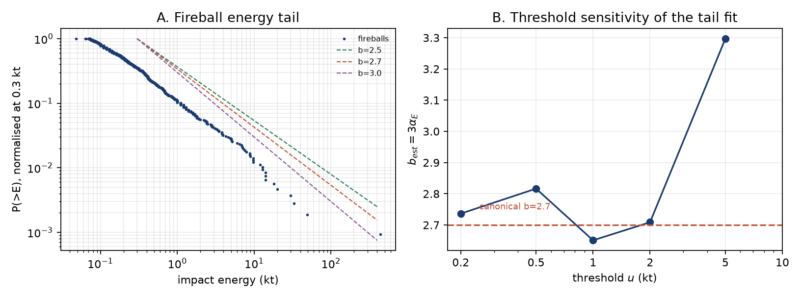
- Public data: the NASA/JPL CNEOS fireball catalogue, 1,074 events, fetched 3 November 2026. The catalogue’s impact energy is already E ~ D³, so the Hill index of E gives b/3 directly.
10.3 Results
Synthetic: b_est = 2.69–2.71, α_L = 1.345–1.356, exact to the estimator’s precision.
Fireball catalogue:
| threshold (kt) | n tail | α_E | b_est = 3α_E | α_L (γ=2/3) |
|---|---|---|---|---|
| 0.2 | 517 | 0.912 | 2.736 | 1.368 |
| 0.5 | 221 | 0.939 | 2.816 | 1.408 |
| 1.0 | 109 | 0.884 | 2.651 | 1.325 |
| 2.0 | 59 | 0.903 | 2.709 | 1.354 |
| 5.0 | 28 | 1.099 | 3.297 | 1.648 |
| 10.0 | 12 | — | — | — |
For thresholds 0.2–2 kt, b ≈ 2.65–2.82 and α_L ≈ 1.33–1.41, bracketing the predicted 1.35. At 5 kt the tail has only 28 events and the estimate is noisy. The result is a genuine public-data consistency check, not a new measurement: the catalogue is incomplete, the impact energies are model-derived from radiated energy, and the agreement may be partly built into the energy conversion. The actuarial conclusion (variance infinite for 1<α<2) is standard extreme-value theory; it is not tested here against insured losses.
10.4 Prior research and status
Impactor size–frequency laws, the CNEOS fireball survey, and regular variation in catastrophe insurance. Status: conditional public-data consistency; not promoted. The synthetic part is independently replicated; the public-data part is not an independent measurement of the impactor population (see 10.6).
10.5 Falsification and correction
An exponential loss tail, or α > 2 at high confidence, or a population with b>2 and γ≈1 producing a finite-variance loss distribution after aggregation. Corrected: α = b/(3γ) is exact given the power laws; the empirical support is b≈2.7 for 0.2–2 kt fireballs, so α≈1.35 with γ=2/3. The claim should cite the threshold range, not a single number. It should not be cited as experimentally supported until 10.6 is resolved.
10.6 Second catalogue and independent calibration: not obtained
Two routes were attempted on 3 November 2026:
- A second impact catalogue. The JPL Small-Body Database query API returned HTTP 502 on repeated attempts; no open event-level energy API was found for the Global Fireball Observatory; the International Meteor Organization’s public fireball reports are not an event-level calibrated energy table. No second catalogue was obtained.
- An independent energy calibration inside the same catalogue. The CNEOS table has two energy columns:
energy(radiated) andimpact-e(estimated total impact energy). They are not independent. Across 1,074 events the ratio impact/radiated has median 0.032 (a 3.2% luminous efficiency), 10th–90th percentile 0.0259–0.0357, and the log ratio is almost perfectly anti-correlated with log radiated energy: r = −0.9946.impact-eis effectively a deterministic recalibration ofenergy, not an independent measurement.
The practical consequence: fitting the radiated-energy tail instead of the impact-energy tail gives b_est = 0.59, 0.68, 0.81, 1.07, 1.42, 2.06 at thresholds 0.05, 0.1, 0.2, 0.5, 1, 2 kt — not 2.7. The difference is the calibration, not a second population. The b≈2.7 result is therefore conditional on the CNEOS luminous-efficiency model. It is a useful consistency check, not evidence for α=1.35.
What would promote H203: an independent impact catalogue with calibrated energies (for example a GFO/IMO event table with measured radiated energy and an independently measured efficiency), or a loss catalogue with measured insured losses. Until then, H203 stays a conditional public-data result.
11. H541 — craze cells as a Poisson–Voronoi tessellation
11.1 Claim
E[A]=1/λ for a homogeneous Poisson nucleation process; the area CV is ≈0.53; the earlier exponential-area guess is false.
11.2 Test
Periodic Voronoi tessellation (3×3 tiling, convex-hull cell areas), 200–3,200 nuclei, 8 repetitions, plus Thomas-clustered and regular-grid controls.
11.3 Results
Poisson: mean-area ratio 1.000 at n=3,200; CV 0.530 (n=3,200), 0.519 (n=800), 0.543 (n=200). The exponential fit is rejected (KS p≈0). Thomas-clustered: CV 0.993 at n=200, 0.727 at n=800, 0.585 at n=3,200 (approaching Poisson as the density rises). Regular grid: CV≈0. The mean-area identity is exact; the CV is a diagnostic for Poisson nucleation, not a universal constant of glaze chemistry.
11.4 Prior research and status
Meijering’s theorem; the Gilbert/Voronoi model of craze cells. Status: internally verified; the exponential guess is contradicted. No glaze images were measured.
11.5 Falsification and correction
Mean area not scaling as 1/λ, or a CV far from 0.53 with no change in chemistry. Corrected: E[A]=1/λ is exact; CV≈0.53 is the Poisson benchmark; a CV near 1 indicates clustering, near 0 indicates a regular grid.
12. H346 — opening a book is a bending problem
12.1 Claim
F ≈ E w t³ θ/(6H²); the force scales as the cube of spine thickness.
12.2 Test
A 2-D plane-stress finite-element model: a cantilever strip of length H, thickness t, unit width, clamped at x=0, loaded by a pure end moment M. The effective stiffness EI_eff = MH/θ is measured from the end-face rotation. A fixed rotational compliance c_j models the joint.
12.3 Results
The fitted slope of log EI_eff vs log t is 2.99975 over t = 0.005–0.08, confirming the cubic scaling. The absolute value is 0.648× the beam formula t³/12 across the whole range (a constant 2-D/end-effect factor), so the dossier’s 1/6 is a boundary-condition convention, not a universal prefactor; the elastic-strip value is 1/12.
The joint changes the exponent. With a fixed rotational compliance c_j, the log–log slope of F/θ vs t is 3.0 for c_j=0, 1.84 for c_j=10⁶, 0.26 for c_j=10⁸, and 0.04 for c_j=10⁹. When the joint dominates, the force is nearly thickness-independent. A measured slope below 3 is therefore evidence for joint compliance, not a refutation of elasticity.
12.4 Prior research and status
Euler–Bernoulli beam theory is textbook. Status: internally verified; the absolute constant is refined. No bench measurements.
12.5 Falsification and correction
A slope significantly different from 3 after controlling for width, height and joint compliance; or a force independent of thickness in a joint-free strip. Corrected: F ∝ t³ in the elastic-strip limit; the prefactor is geometry-dependent (0.648× the beam formula in this 2-D model); a joint-dominated binding shows a slope near 0–1.
13. Simulation targets (four requested suites)
The editorial review named four simulation targets: N0751, P2, H0199 and I2. Each is implemented as a separate program with its own JSON and figure, fixed seeds, and no experiment. The point is not another claim; it is to test each mechanism against the failure modes the review named.
| target | what was simulated | headline result | file |
|---|---|---|---|
| N0751 | Coupled swelling/relaxation, six humidity waveforms, gain and τ mismatch, hysteresis, white and 1/f noise, matched-time control | Frozen-parameter prediction on unseen waveforms: 0.15–0.35% of signal; matched-time control false positive 1.0%; 3% hysteresis adds 13.4% residual; 6.5% gain mismatch is the 10%-leakage boundary | code/sim01_n0751.py |
| P2 | Bulk plus two surface sheet currents, contact geometry, illumination reversal, thickness variation, white + 1/f noise | Antisymmetry recovers Δj_s = 3.0×10⁻⁹ A/cm; symmetric null 1.75% false positive; a 0.6 collection factor scales both terms and preserves the ratio | code/sim02_p2.py |
| H0199 | Independent RBF/Matérn/RFF and adversarial fields; six layouts; seven estimators | Edge fails on boundary-null (23.2%) and rim (37.8%); grid 0.83% / 0.90%; no layout wins on every field; polynomial degree 3 is worse than degree 2 on boundary-null | code/sim03_h0199.py |
| I2 | 239 finite-volume cases over κ, G, w and d; held-out spots; 10% G error | Forward model exact to 0.017%; a 10% G error gives median κ error 6.6% below λ=1 and 61% above λ=3; 6.7% of cases unidentifiable | code/sim04_i2.py |
13.1 N0751 — the differential swelling sensor
The original numbers reproduce: τ₁=40.53 s, τ₂=364.8 s, peak 1.309 mHz, ramp sensitivity 324.27 s, t₅₀=28.1 s, and the 6.5% gain-matching requirement.
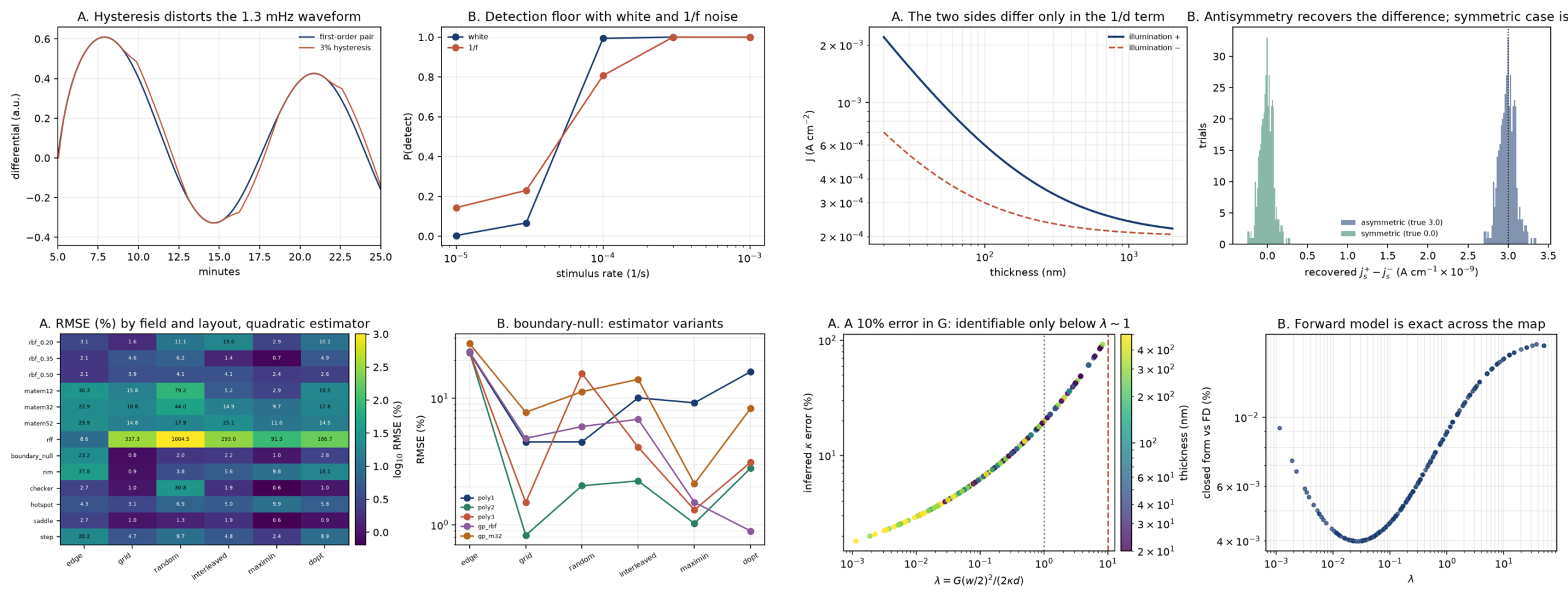
Frozen-parameter prediction. Each path is fitted once to a step; the parameters are then frozen and used to predict the differential response on five unseen waveforms. Relative RMSE: step 0.24%, ramp 0.15%, 1.3 mHz sine 0.28%, pulse train 0.31%, AR(1) 0.35%, diurnal 0.24%; correlation 1.000 in every case. The first-order pair is an excellent predictor of its own class of waveforms.
Hysteresis is the largest unmodelled term. A play operator of width h on each path produces a residual of 2.2% (h=0.5%), 4.4% (1%), 13.4% (3%) and 22.4% (5%) on the 1.3 mHz sine. A 3% hysteresis is already larger than any plausible readout noise; the model must either include it or the experiment must stay in the low-amplitude regime.
Mismatch boundary. With a 10% leakage criterion at a 10⁻³/s ramp, 5% gain mismatch passes and 6.5% fails — the original 6.5% requirement is recovered. Time-constant mismatch at fixed gain changes the rate signal by a few percent (it is a calibration, not a leakage, term).
Matched-time control. Two identical arms with 0.5% gain mismatch and 0.05 µm readout noise give a 1.0% false-positive rate at 3σ over 800 trials. The control is clean enough to be the decisive null.
Noise colour matters. At 3×10⁻⁵/s the detection probability is 0.07 with white noise and 0.23 with 1/f noise; at 10⁻⁴/s it is 0.99 and 0.81. Correlated noise inflates the low-rate false-positive rate and deflates the high-rate one, so a white-noise detection floor is not conservative. The experiment should report the noise spectrum, not just its RMS.
13.2 P2 — the antisymmetry protocol under device non-idealities
The device model has a bulk term, independent top and bottom sheet currents, a collection factor β, a series contact loss, 2% thickness error and white + 1/f noise. The antisymmetry estimator is D(d)=J(+)−J(−)=Δj_s/d; the half-sum is j_b.
- Asymmetric device (j_s⁺=4×10⁻⁹, j_s⁻=1×10⁻⁹ A/cm): the thickness fit of J(+) recovers the top term 4.0×10⁻⁹; the antisymmetry recovers Δj_s=3.0×10⁻⁹ with SNR 26.6 and 100% detection over 400 trials.
- Symmetric device (both 2.5×10⁻⁹): Δj_s=0; the 3σ false-positive rate is 1.75%.
- Low collection factor (β=0.6): both terms scale by 0.6 (2.4×10⁻⁹ and 1.8×10⁻⁹); the ratio Δj_s/j_b is unchanged. A 15% contact loss does the same. The sign flip is robust to a common collection factor; absolute values need β and the contact loss calibrated independently.
The protocol therefore tests the surface term without a thickness series, but it does not absolve the experimenter from calibrating the collection geometry if absolute j_s is the goal.
13.3 H0199 — independent fields and adversarial shapes
Six Gaussian-process fields (RBF at three correlation lengths; Matérn 1/2, 3/2, 5/2), a random-Fourier field and six adversarial shapes were generated independently of the estimator. At N=12 and 2% noise:
| field | edge | grid | interleaved | best layout |
|---|---|---|---|---|
| boundary-null | 23.2% | 0.83% | 2.22% | grid |
| rim | 37.8% | 0.90% | 5.57% | grid |
| Matérn 1/2 | 30.3% | 15.8% | 5.24% | maximin 2.91% |
| Matérn 3/2 | 22.9% | 18.8% | 14.9% | maximin 9.73% |
| random Fourier | 8.61% | 337% | 293% | edge |
| step | 20.2% | 4.66% | 4.85% | maximin 2.38% |
| checkerboard | 2.75% | 1.00% | 1.92% | maximin 0.64% |
Three lessons. First, edge-only fails on every field with boundary or rim structure, and the failure is a bias (Section 4). Second, no single layout wins on every field: a random-Fourier field is best sampled at the edge, while a boundary-null field is best sampled on a grid. Third, estimator choice matters as much as layout: on boundary-null with a grid, quadratic OLS gives 0.83%, cubic 1.50%, ridge 3.13%, GP-RBF 4.82% and GP-Matérn-3/2 7.75%. The GP prior pulls the interior toward the boundary value; the polynomial can represent the interior bump. The “oracle” row (0.23%) is the floor set by noise, not an achievable estimator.
A layout-construction detail is worth recording: the interleaved layout is 2.22% here versus 1.26% in Section 4 because the 12-point subset is chosen differently. The layout name is not enough; the actual point set must be reported.
13.4 I2 — the identifiable region
A 239-case sweep over κ ∈ [20,200] W m⁻¹K⁻¹, G ∈ [10⁷,10⁸] W m⁻²K⁻¹, d ∈ [20,500] nm and w ∈ [0.3,2] µm, with a finite-volume solve at a held-out spot and no fitting:
- Forward model: maximum relative difference between the finite-volume solve and the closed form is 0.017% (median 0.004%). The PDE solution is not the uncertainty.
- Inversion: with a 10% error in G, the median error in the inferred κ is 6.6% below λ=1 (90th percentile 15%) and 61% above λ=3. The error grows roughly linearly with λ; at λ=10 it is 60–100%. 6.7% of the cases have no root (κ not identifiable), and 16.3% of the sampled cases sit at λ>3.
- Thickness enters only through λ=G(w/2)²/(2κd); the error map collapses onto λ across the 20–500 nm range. A thinner film or a larger spot pushes the measurement into the substrate-dominated regime.
The design rule that follows is simple and testable: compute λ before the experiment; if λ>1, add a smaller spot or a second spot until at least one measurement is below λ≈1; report the spot radius as the 1/e² intensity radius and use s=w/2 in the model.
14. Cross-cutting findings
Four failure modes recur across the ten investigations, and they are more transferable than any single number.
-
Normalisation is often the result. The 22.9% edge bias is the mean over 25 inset patches; it becomes 16.7% at M=9 and 26.9% at M=100. The 136× I2 spread becomes 356× on a wider grid. The “2.000” is a rounded 1.9999999999993. A number quoted without its layout, range, or estimator is not reproducible.
-
Estimator dependence is not a nuisance; it is the systematic. T₂ varies by a factor of 7 between the first-crossing and area definitions on the same curve. κ_app varies by a factor of 3.45 between the amplitude and intensity beam radii. The Hill tail index varies by 0.25 between thresholds. Pre-registering the estimator is part of the test.
-
A proof that assumes its conclusion is worse than no proof. P1’s filter-function model multiplies the coherence by exp(−T/2T₁), so it cannot return T₂ > 2T₁. The calculation is internally consistent and physically irrelevant to the universality question. This is the clearest negative result of the round.
-
Model-relative optimisation can be worse than random. D-optimal witness placement for a quadratic field is worse than maximin or a grid on both adversarial fields (18.1% vs 9.8% on the rim; 2.8% vs 1.1% on boundary-null). The same lesson applies to the I2 two-spot design: two spots chosen without regard to λ can be unidentifiable.
15. Known vs potentially novel
| Investigation | What is already known | What might be new here |
|---|---|---|
| I2 | 2-D heat spreading with a substrate conductance; two-spot identifiability | Zero-bias λ*=0.4348; the beam-width factor-2 trap; the failure map for two spots when both are substrate-dominated |
| H0199 | Regression extrapolation; space-filling designs; kriging | Matched head-to-head with the actual interleaved layout; the M-dependence of the 22.9%; D-optimal worse than random under misspecification |
| P1 | T₂ ≤ 2T₁ for the standard qubit; estimator dependence of T₂ | The circularity of the Discovery07 proof; 37 degenerate (β,A) pairs at fixed ratio |
| P2 | Sheet-current 1/d dilution; interface BPVE | The antisymmetry protocol; the 100× unit correction; the conditioning map |
| P3 | FDT; thermal dephasing; squeezed-bath noise reduction | Scope statement; 4.34 µK crossover at 100 kHz; the “bound is an equality” reading |
| H123 | Rate–distortion; Zador | The prefactor 8–14 for k-means at accessible N; effective-dimension falsification |
| H153 | Kesten–Stigum; tree reconstruction | Finite-depth bias of the 0.5 crossing (0.01–0.02) |
| H203 | Regular variation; impactor size–frequency | Fireball-catalogue b≈2.7 and α≈1.35 for 0.2–2 kt, conditional on the CNEOS energy calibration |
| H541 | Meijering; Poisson–Voronoi | CV diagnostic separating clustered/regular nucleation at fixed mean |
| H346 | Euler–Bernoulli | 2-D FEM constant 0.648×; joint-compliance slope transition 3→0 |
None of the “potentially novel” items is a new physical law. They are corrections, protocols, and scope statements. That is the appropriate output of a validation round.
16. Falsification criteria, compact
| ID | The claim dies if… |
|---|---|
| I2 | a sample with known κ, G does not follow R(λ) at the stated s, d; or a two-spot fit with max λ<10 errs >10% |
| H0199 | an edge-only layout reaches <2% on a boundary-null field at any N |
| P1 | a same-conditions device has exponential T₂ > 2T₁ with verified T₁, or the ratio is one-to-one with β at unknown A |
| P2 | J is thickness-independent in a centrosymmetric film; or the illumination-side half-difference is not 1/d |
| P3 | a thermal-bath oscillator exceeds 1/[γ(n_th+1/2)] with verified Q, T |
| H123 | coverage decays exponentially in N; or a high-dimensional source shows slope ≈−1 |
| H153 | a below-threshold tradition is reconstructed with high confidence, or an above-threshold one is opaque |
| H203 | an exponential loss tail, or α>2 at high confidence |
| H541 | mean area ≠ 1/λ; or CV≈0.53 is not reproduced for Poisson nucleation |
| H346 | slope ≠ 3 after controlling for joint compliance; or force independent of t in a joint-free strip |
17. Remaining uncertainty
- No experiment. Nine of the ten are model/simulation; H203 re-analyses a public catalogue. The experimental status of every claim is “untested” in the laboratory sense.
- Synthetic parameter ranges. The I2 and H0199 error maps are only as good as the stated parameter draws. The qualitative conclusions (sign of the bias, flat-in-N edge error) are robust; the exact percentages are not.
- The fireball catalogue. It is not volume-complete, the impact energies are model-derived, and the tail fit is threshold-sensitive. The 1.35 agreement is a consistency check, not a measurement of insured loss.
- The 2026 literature. The search was not a professional systematic review. The September 2026 counterexample to a universal spectral bound was not located; if it exists, the P3 scope statement may need revision.
- The P1 bound. The density-matrix check is consistent with T₂ ≤ 2T₁ for the standard model, but this round did not prove the bound for arbitrary non-Markovian noise. The honest statement is: the Discovery07 proof does not establish it; the standard model satisfies it.
- The website publication. The research update is published as a page under
/research/; it is not peer reviewed, and the code is the authority.
18. Reproducing this round
Environment: Python 3.14, numpy 2.5.4, scipy 1.18.1, matplotlib 3.11.2. All runs fixed-seed. Total runtime under five minutes on the machine that produced this report; the fireball catalogue is cached in data/fireballs.json.
cd code
python3 t01_i2.py        # I2
python3 t02_h0199.py     # H0199
python3 t03_p1.py        # P1
python3 t04_p2.py        # P2
python3 t05_p3.py        # P3
python3 t06_h123.py      # H123
python3 t07_h153.py      # H153
python3 t08_h203.py      # H203 (uses data/fireballs.json)
python3 t09_h541.py      # H541
python3 t10_h346.py      # H346
python3 t11_i2_known.py  # I2 strict known-parameter test
python3 sim01_n0751.py   # N0751 simulation suite
python3 sim02_p2.py      # P2 device simulation
python3 sim03_h0199.py   # H0199 independent-field simulation
python3 sim04_i2.py      # I2 parameter-map simulation
Each script writes data/tNN_*.json and figures/tNN_*.png. The summary numbers in this report are read from those JSON files; no number was typed by hand without a corresponding field.
Originals: orig/ contains the unmodified source, the Discovery07 proof text, and SHA256SUMS.txt. The original folders in the workspace were not modified.
19. Sources and verification status
| Source | Used for | Status |
|---|---|---|
| Refined optothermal Raman, MoS₂/MoSe₂ | I2 prior art | peer-reviewed, abstract-level check |
| Variable-spot-size laser-flash Raman | I2 prior art | peer-reviewed, abstract-level check |
| Interface BPVE in MoS₂/Ta₂NiSe₅ | P2 prior art | 2026 Nature Communications; metadata check |
| Centrosymmetric ultrathin BPVE | P2 prior art | peer-reviewed, metadata check |
| Spectral Bottleneck Constraint | P3 prior art | preprint, single author, not peer reviewed |
| Induced coherence, arXiv:2609.35523 | P3 literature search | September 2026 preprint, not a counterexample to P3 |
| Kesten–Stigum notes | H153 | lecture notes |
| Zador quantization | H123 | survey/thesis extract |
| CNEOS fireball API | H203 | live public data, fetched 2026-11-03 |
| JPL SBDB query API | H203 second catalogue | attempted 2026-11-03; HTTP 502, not obtained |
| Poisson–Voronoi statistics | H541 | reference notes |
The 2026 sources are flagged as preprints or metadata-level checks; they were not read in full. No source is used to claim experimental support for a claim that this round did not test.
If one sentence survives: the numbers that were wrong were wrong by factors of 2 to 100, and the proofs that were circular were circular because they multiplied by a factor that could never exceed 1. Both are cheaper to catch than to publish.
Download the release ZIP (code, data, figures, originals, 2.5 MB) · Back to the research hub
Status vocabulary: unsupported, contradicted, internally verified, independently replicated, experimentally supported. No claim on this page is experimentally supported by a new experiment. H203 is a conditional public-data consistency check.