Bursts increase backlog without changing this queue’s load threshold
Independent mathematical/computational model check · 30 October 2026 · not peer reviewed.
The proposed variance-driven instability mechanism does not hold in the fixed-capacity point queue tested here. Exact arithmetic gives an under-capacity burst pattern that repeatedly drains. In the stochastic family, larger bursts increase backlog and tail exceedances, while the strict load-based stability condition remains in force. This result concerns the stated model; it is not empirical proof about road traffic, a validation of all traffic models, or a new queueing theorem.
The original “Congestion Onset Is Variability, Not Volume” hypothesis remains unchanged. This is an additive test report. Its broader predictions about real-road breakdown and the relative cost effectiveness of smoothing versus capacity additions remain untested.
Question, plan and observation convention
The narrow claim examined is that high arrival variance can make a below-capacity queue mathematically unstable even when its mean input is unchanged. We specify a single infinite-buffer, work-conserving queue with fixed capacity C=1:
Q[t+1] = max(0, Q[t] + A[t] − 1).
Q is backlog after same-cycle service. It is not workload just before service, a measured traffic jam, or an individual vehicle’s travel delay. The queue starts empty. The constant-input comparison uses fractional work, not fractional vehicles.
The full plan was saved locally at 2026-10-30T16:31:08.992077+00:00 before the experiment began at 2026-10-30T16:32:19.162913+00:00. It was not changed during the run. This is a locally saved pre-execution plan, not an independently registered protocol. No conditions, seeds, horizons or outcomes were selected after observing results.
Exact matched-mean calculation
Both arrival streams supply four work units in five cycles, mean 0.8, below capacity 1:
| Arrival stream | Arrival variance over a five-cycle period | Repeating after-service backlog | Mean backlog | Maximum after-service backlog |
|---|---|---|---|---|
| Constant fluid input 0.8 each cycle | 0 | 0,0,0,0,0 | 0 | 0 |
| Bursts 4, 0, 0, 0, 0 | 2.56 | 3,2,1,0,0 | 1.2 | 3 |
The burst stream’s peak before service is4. Its five-cycle map from any nonnegative initial backlog q is:
F(q) = max(0, q − 1).
To see this, the burst adds four and the first service removes one, producing q+3; the next four services reduce that to max(0,q−1). Thus each complete period reduces any excess initial backlog, and the initially empty queue repeats a bounded cycle. The 100-cycle exact trace and period-map checks use rational arithmetic. The map is the mathematical argument; observing a short simulation alone would not prove boundedness.
This example distinguishes temporary backlog from instability. It contradicts a universal “bursts must destabilize an underloaded fixed-service queue” explanation. A single example does not refute an existential claim about some real road network with additional mechanisms.
Stochastic design and uncertainty
Arrivals are independently drawn as A=b with probability ρ/b and A=0 otherwise. Capacity remains1. Loads are 0.50, 0.80, 0.95 and 1.05; batches are 1, 2, 4 and 8. The requested cell ρ=1.05,b=1 is infeasible because its Bernoulli probability would be 1.05; it was explicitly excluded in the plan rather than clipped.
The 15 valid conditions each have 64 separately seeded replicates of 100,000 cycles, with 20,000 burn-in cycles and 80,000 measured cycles. This is 960 runs and 96,000,000 simulated cycles. The deterministic seed rule and every seed are public in the plan and replicate results. Checkpoints for every run at 0 and every 5,000 cycles are also retained. Individual per-cycle random draws are not stored; the seeds and code reproduce them.
Intervals are the replicate mean ±2 times its Monte Carlo standard error, approximately 95% intervals. Standard errors come from 64 replicate estimates, not from treating the 80,000 correlated time points as independent samples. These intervals describe finite-run Monte Carlo precision, not uncertainty about real traffic. They are not simultaneous inference across all displayed metrics. Starting empty and using finite burn-in can still introduce bias.
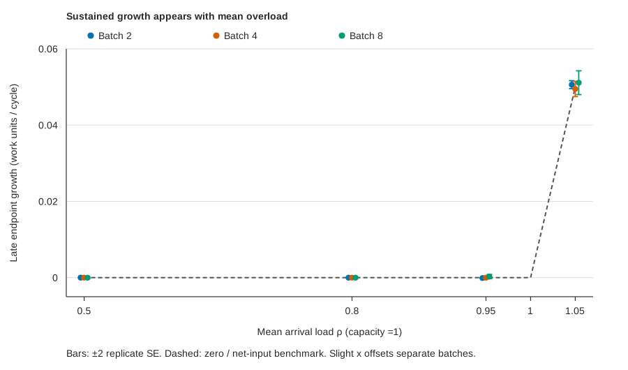
“Late growth” is (Q[100000] − Q[50000]) / 50000. Nonzero
finite-run slopes are not stability tests. For example, ρ=0.95,b=2 has a
small negative late-growth interval excluding zero; it was retained
without rerunning or recoding. A zero observed tail and a degenerate
zero interval mean no such tail event was seen, not
proof that its true probability is zero.
Analytic context and benchmark
For independent bounded increments A−1 with strict negative mean, the reflected queue has a stationary distribution. Glynn and Zeevi’s primary paper gives this result and a finite-second-moment stationary-mean bound in §5.1, printed p.208. The classic Loynes paper also distinguishes subcritical, supercritical and critical behavior. We do not assert a universal rule at the untested boundary ρ=1.
For this particular bounded, integer batch family under ρ<1, the stationary after-service mean can be derived exactly:
E[Q] = ρ(b−1) / (2(1−ρ)).
Here is the moment balance, rather than an appeal to a
continuous-time approximation. Write U=1 only when Q=0 and A=0. Then
Q′=Q+A−1+U, stationarity gives E[U]=1−ρ, and
(Q′)²=(Q+A−1)²−U. Independence gives
0 = 2(ρ−1)E[Q] + E[(A−1)²] − E[U] = 2(ρ−1)E[Q] + ρ(b−1).
The bounded independent negative-drift model has finite stationary moments, justifying these balances. At fixed ρ, arrival variance is ρb−ρ² and the exact mean backlog increases with b, even though the strict load condition does not change. This is a model-specific benchmark and classical queueing behavior, not a claim of novelty.
For ρ>1, cumulative demand eventually exceeds cumulative potential service under the model’s independent arrivals. Finite runs illustrate the positive net input; they do not create a stationary mean. The reported overload backlog averages below are finite-horizon quantities.
Results
At load 0.80, batch 2, 4 and 8 mean backlogs were 2.008, 5.972 and 13.897; the corresponding analytic stationary means are 2, 6 and 14. Batch 1 has zero after-service backlog by construction. At load 0.95 and batch 8, the mean was67.166 with approximate Monte Carlo interval[62.768,71.564], compared with the analytic mean 66.5.
At load 0.80 and batch 8, the observed fraction with at least 10 backlog units was47.88%; at load 0.95 and batch 8 it was84.11%. These are queue-threshold exceedances, not measured road-breakdown probabilities. All 12 underloaded condition means had their analytic benchmark inside the reported approximate Monte Carlo interval; this is a numerical consistency check, not the proof of stability.
Overloadρ=1.05 produced mean late growth 0.050610, 0.049486 and 0.051127 work units/cycle for batches 2, 4 and 8, respectively, around the net-input value 0.05. The full outcomes, including zeros, non-supportive finite trends and the infeasible cell, are retained.
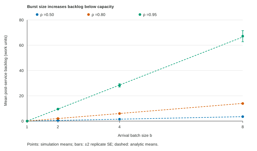
| Load ρ | Batch b | Mean backlog [approx MC interval] | Analytic stationary mean | Observed Q≥10 | Observed Q≥100 | Late growth [approx MC interval] |
|---|---|---|---|---|---|---|
| 0.50 | 1 | 0.000 [0.000, 0.000] | 0 | 0.0000% | 0.0000% | 0.000000 [0.000000, 0.000000] |
| 0.50 | 2 | 0.500 [0.498, 0.502] | 0.5 | 0.0014% | 0.0000% | 0.000002 [-0.000005, 0.000008] |
| 0.50 | 4 | 1.501 [1.491, 1.510] | 1.5 | 1.4430% | 0.0000% | -0.000006 [-0.000027, 0.000016] |
| 0.50 | 8 | 3.516 [3.484, 3.547] | 3.5 | 12.3289% | 0.0000% | -0.000024 [-0.000063, 0.000015] |
| 0.80 | 1 | 0.000 [0.000, 0.000] | 0 | 0.0000% | 0.0000% | 0.000000 [0.000000, 0.000000] |
| 0.80 | 2 | 2.008 [1.993, 2.024] | 2 | 1.8089% | 0.0000% | -0.000010 [-0.000030, 0.000010] |
| 0.80 | 4 | 5.972 [5.911, 6.032] | 6 | 22.2530% | 0.0000% | -0.000008 [-0.000058, 0.000043] |
| 0.80 | 8 | 13.897 [13.657, 14.137] | 14 | 47.8847% | 0.1815% | -0.000015 [-0.000096, 0.000066] |
| 0.95 | 1 | 0.000 [0.000, 0.000] | 0 | 0.0000% | 0.0000% | 0.000000 [0.000000, 0.000000] |
| 0.95 | 2 | 9.491 [9.227, 9.754] | 9.5 | 36.4581% | 0.0000% | -0.000105 [-0.000175, -0.000035] |
| 0.95 | 4 | 28.254 [26.932, 29.576] | 28.5 | 69.5480% | 3.2680% | -0.000029 [-0.000232, 0.000173] |
| 0.95 | 8 | 67.166 [62.768, 71.564] | 66.5 | 84.1078% | 22.6942% | 0.000279 [-0.000281, 0.000839] |
| 1.05 | 2 | 3020.644 [2964.279, 3077.009] | not stationary | 100.0000% | 100.0000% | 0.050610 [0.049566, 0.051654] |
| 1.05 | 4 | 3124.474 [3023.059, 3225.889] | not stationary | 100.0000% | 100.0000% | 0.049486 [0.047482, 0.051490] |
| 1.05 | 8 | 3186.173 [3041.805, 3330.541] | not stationary | 100.0000% | 100.0000% | 0.051127 [0.048005, 0.054250] |
Rows below capacity compare stationary benchmarks with finite-run means. Overload rows have no stationary mean. Tail percentages are observed measurement-window fractions; zeros are observations, not established absent tails. Approximate intervals use independent-replicate standard errors as preplanned.
Secondary comparison recognized after the run
The periodic stream 4, 0, 0, 0, 0 and independent batch 4 arrivals at load 0.8 share the same mean 0.8 and marginal variance 2.56 (over the cycle for the periodic stream). Yet the periodic mean backlog is 1.2, whereas the independent-input analytic mean is 6 and the simulated estimate is 5.972. Temporal arrangement therefore matters too; mean and variance alone do not specify backlog. This is a secondary analytic comparison of existing cases, recognized after execution, not an additional preplanned test. No new simulation was run for it.
Which parts of the original hypothesis were tested?
| Statement or prediction | Outcome of this work |
|---|---|
| Higher variance alone changes stability at a fixed below-capacity mean in this point queue | Not supported under the specified independent bounded-arrival/fixed-service assumptions. The exact periodic example is bounded, and the negative-drift condition covers all tested stochastic below-capacity cells. |
| Burstier input can create more temporary backlog at the same mean | Supported in these explicit model comparisons. It does not imply unbounded growth. |
| P1: variability predicts urban congestion onset better than volume/capacity | Not tested: no road observations or predictive comparison. |
| P2: matched-mean roads differ in physical breakdown probability | Not tested: backlog thresholds in a point queue are not road breakdown. |
| P3: smoothing outperforms equivalent-cost capacity additions | Not tested: no intervention cost model or capacity experiment. |
No source article or earlier publication has been replaced. A responsible refinement is: in a fixed-service queue, variability can substantially increase delay burden below capacity, while load remains central to stability; whether road networks behave differently requires empirical or richer network tests.
Limits
The model has infinite storage, fixed capacity and independent bounded batches. It excludes capacity drop, spillback, interacting intersections, route choice, signals with state-dependent service and time-varying demand. Physical gridlock can involve exactly those mechanisms. No traffic dataset was calibrated, and nothing here establishes a transport policy recommendation. Statistical stability is a stationary-distribution concept; it does not require every random sample path to stay below one fixed bound forever. Only the deterministic periodic example is proved pathwise bounded.
No independent preregistration or peer review is claimed. The simulation is a consistency illustration with finite-horizon and burn-in limits; the exact map and the stated mathematical conditions carry the narrow model conclusion.
Reproduce and inspect
Python 3 standard library only; no installation, credentials or network needed:
python3 run_experiment.py --plan plan.json --output-dir rerun-resultsUse a new output directory; the runner refuses to overwrite computed
results. Python version and code/plan hashes are in run metadata. Reports and SVG figures can
be regenerated from results with build_report.py (report
rendering additionally uses an existing Pandoc installation; the
experiment itself does not).
- Pre-execution plan, plan commit record, experiment code, report/figure code.
- Exact deterministic results, trace CSV, period-map CSV.
- Condition summaries CSV and JSON.
- Every replicate CSV and JSON, including seeds.
- All stored checkpoints CSV and JSON.
- Complete result object, primary-source context, original hypothesis HTML as text.
- Independent computational audit: checked hashes, seed rules, all summary values, and three preselected independent replays. This is a computation check, not external peer review or traffic validation.
- File hashes and provenance.