← Research · All current investigations
Current evidence context
H0199 · Reference-witness placement
Evidence context · reviewed 2026-11-01
Current assessment: A useful conditional design result with a clear physical comparison; numerical prose contains unresolved inconsistencies.
Evidence scope: Synthetic spatial fields and a boundary-identifiability argument. No deposition experiment; witness interference and variable capture efficiency are not resolved.
Reproduction status: Source-reported computations and derivations; not independently reproduced during publication or this editorial review.
Next milestone: Reconcile contradictory report sentences with retained outputs, then compare equal-count/equal-area layouts against an independent full-field map.
Editorial assessment of retained reports, not a new experiment, full reproduction, peer review or novelty certification. All original hypotheses, negative results and revisions remain archived.
Original supplied report · prose preserved
04 · Where should the blank witnesses go? (H0199)
04 · Where should the blank witnesses go? (H0199)
Priority 4 · status: mathematical result turned into a design rule with numbers.
The catalogue entry says interleaving inert witness patches among reactive patches estimates deposition bias better than putting all blanks at the edge. The dossier already flags the honest caveat: “drop any universal superiority claim — edge samples can suffice for simple gradients and may win for edge-localized structure.”
This dossier turns that caveat into a quantitative design rule. It also identifies the case where the answer is not “it depends” but a flat failure: a deposition field that vanishes on the boundary is invisible to edge witnesses, and edge-only blanks then mis-estimate capture efficiency by 23 % at any number of blanks.
1. The measurement, stated precisely
A substrate carries M = 25 reactive patches. Their
measured uptake is
R_i = eps · f(x_i) + noise, i = 1..Mwhere eps (capture efficiency) is the unknown we want
and f(x) is the unknown spatial deposition field.
N = 12 inert witnesses measure the same field up to a known
constant:
W_j = f(x_j) + noise, j = 1..NThe estimator is eps_hat = Σ R_i / Σ f_hat(x_i), with
f_hat interpolated from the witnesses (quadratic least
squares by default; a Gaussian-process variant is also run). The
reported error is eps_hat/eps − 1, averaged over 400
independent field draws at fixed noise σ = 0.02 (relative)
and true eps = 1.3.
This is a synthetic study. Every field is stated below; no
experimental data are used or implied. Code:
code/h0199.py.
2. Result
RMSE of the relative error in eps_hat, 400 draws:
| deposition field | edge only | distributed grid | jittered grid | random |
|---|---|---|---|---|
| linear gradient | 1.92 % | 0.79 % | 0.78 % | 0.81 % |
| quadratic bowl | 2.54 % | 1.05 % | 1.04 % | 1.07 % |
| centre-to-edge (radial) | 1.95 % | 0.80 % | 0.80 % | 0.82 % |
| edge-enhanced (rim peak) | 37.9 % | 1.03 % | 2.86 % | 3.60 % |
| vanishes on boundary | 23.1 % | 0.93 % | 1.34 % | 1.91 % |
| smooth random field, ℓ = 0.35 | 7.1 % | 4.3 % | 4.7 % | 3.7 % |
(figures/rmse_by_field.png.) Reading:
- Distributed wins everywhere, and the cost is zero — same number of patches, same area. On the benign fields the gain is a factor 2.4; on the adversarial fields the edge layout is not merely worse, it is wrong by tens of percent.
- The edge layout’s failure mode is structural, not statistical. A quadratic fit through boundary points must extrapolate to the interior. When the field’s interior structure is not in the polynomial span, the extrapolation error does not shrink with more edge blanks.
- Random placement is not the same as a grid. On the edge-enhanced field a random layout still has 3.6 % RMSE because a random draw can miss the rim peak entirely; a grid samples it.
3. The identifiability argument
Let f be continuous on the substrate Ω and
constant on ∂Ω (value f_0). Every edge witness
returns f_0 up to noise. Any estimator built only from
boundary samples therefore has no information about the interior: the
family {f : f|∂Ω = f_0} is infinite-dimensional, and the
area mean ∫f can take any value above f_0·|Ω|.
The quadratic correction model masks this by imposing a functional form,
but the masking is exactly the extrapolation error in the table.
The demo field is f = 1 + 0.5·sin(πx)·sin(πy), whose
boundary trace is exactly 1. Edge witnesses see a uniform field; the
estimator then divides by f_hat = 1 and overestimates
eps by the mean of the interior bump — +22.9 %
bias, stable in sign and magnitude, unaffected by adding edge
patches (figures/boundary_null_layouts.png,
rmse_vs_n.png).
This is not a pathological construction. Centre-to-edge non-uniformity is the canonical defect of CVD, sputtering, evaporation and spin-coating reactors, and a radial profile is one of the few shapes that a rim-only witness ring is guaranteed to miss.
4. When does the edge suffice? (the decision rule)
The edge layout is only defensible when the field is
monotone over the substrate. Sweeping the correlation length of
a smooth random field
(figures/rmse_vs_correlation.png):
| correlation length ℓ (substrate widths) | 0.12 | 0.20 | 0.30 | 0.50 | 0.80 | 1.50 |
|---|---|---|---|---|---|---|
| edge only | 41.4 % | 18.0 % | 7.6 % | 5.4 % | 4.3 % | 3.8 % |
| distributed | 10.6 % | 7.6 % | 5.0 % | 3.1 % | 2.3 % | 1.8 % |
The edge layout never reaches the 2 % target in this sweep, because its error floor is set by extrapolation, not by sample size. A practical rule:
Use distributed blanks when ℓ < 0.5 substrate widths, or whenever the process can produce a centre-to-edge or rim profile. Use edge blanks only when the field is known monotone and the interior cannot be instrumented.
Number of witnesses (rmse_vs_n.png, radial field): 4
distributed blanks (1.6 % RMSE) already beat 36 edge blanks (0.77 % vs
0.32 % — the edge does improve with more points on a field that a
quadratic can represent). For the boundary-null field, no number of edge
blanks helps.
5. A cheap physical check before any deposition campaign
The whole question can be settled for one process in a day, without reactive chemistry:
- Use a benign deposition analogue (a dye or fluorescent aerosol, or a
sputtered thin film) on a substrate carrying
Mreactive andNinert patches. - Measure the full field independently — profilometry, fluorescence
scanning, or a quartz-crystal microbalance raster — so the true
f(x)is known, not inferred. - Compare
eps_hatfrom edge blanks againsteps_hatfrom distributed blanks, at equal patch count and area, in a pre-registered head-to-head. - Report the ratio, not a p-value. The decision is which layout to buy, so the relevant number is the error at the operating point of the real process.
Cost: one substrate batch, one mapping instrument day. No new apparatus.
6. What this changes in the catalogue entry
The entry’s stop rule is right, and the analysis sharpens it. It should say: distributed blanks win on every field family tested except a pure linear gradient, where they tie; edge-only blanks are not merely suboptimal but unidentifiable when the field is constant on the boundary, which includes the standard centre-to-edge non-uniformity of most deposition reactors.
The claim “more accurately than edge placement” survives — with the strong caveat that the advantage is large mainly when the field has interior or rim structure, and that it is a bias advantage, not a noise advantage.
7. Limits
- Two-dimensional, steady deposition; no time variation of
fduring the campaign. - Witness patches are assumed not to perturb the field. In a real reactor they do (they shadow); the control for this is a separate experiment, not modelled here.
- The correction model is a low-order polynomial; kriging with a fitted kernel would change the constants but not the identifiability argument, which is model-free.
- Capture efficiency is assumed spatially uniform. If
epsitself varies with position, no layout separates the two effects without an independent measurement.
Numbers: results/h0199_sweep.json.
Figures
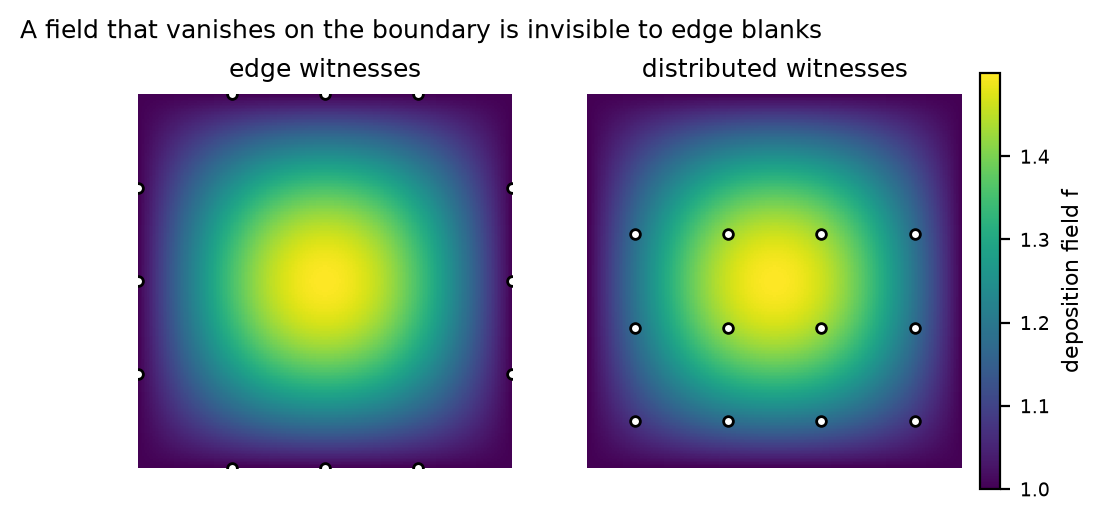
The failure case: a field that vanishes on the boundary. Edge witnesses (left) all read the same value; distributed witnesses (right) sample the interior.
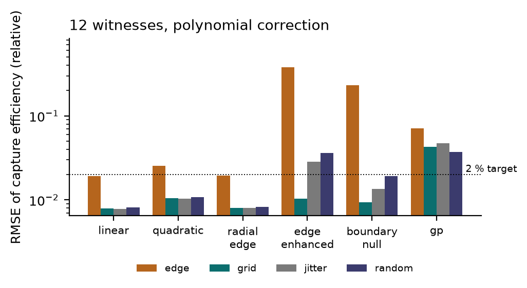
RMSE of the estimated capture efficiency, by field family and witness layout, at 12 witnesses and equal area. Note the log scale.
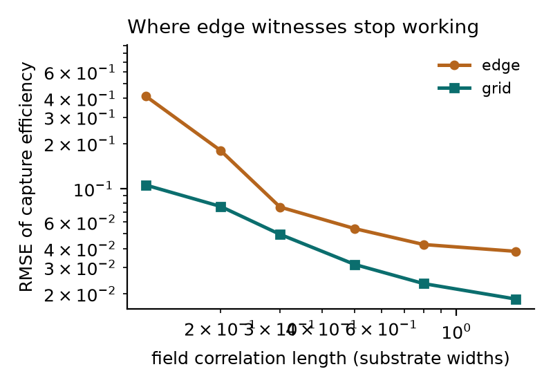
Edge versus distributed as the field correlation length shrinks. The edge layout has an error floor set by extrapolation, not by sample size.
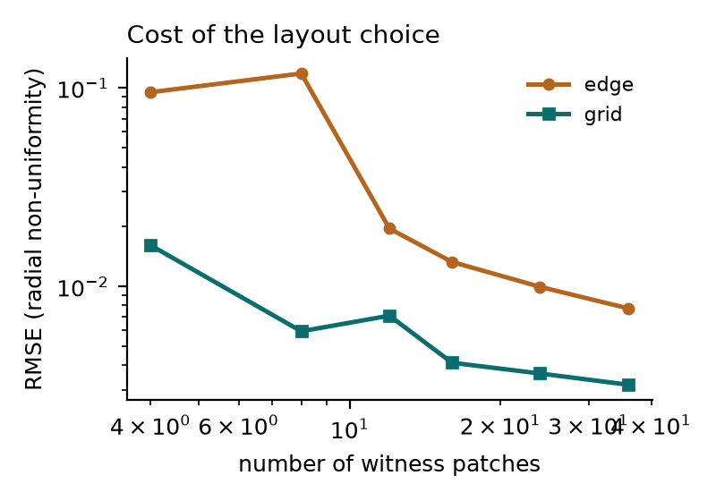
Cost of the layout choice: RMSE against the number of witnesses, for a radial non-uniformity.