A Force Standard for Robot Hands

A traceable uncertainty chain for absolute force and stiffness in the soft-tissue band

Direction: incoprea Frontier Idea #24. A metrology study, not a device. It asks what a tactile sensor’s absolute force and stiffness numbers are worth in newtons and kilopascals — an uncertainty statement no tactile paper publishes.

Provenance. Every number is [ASSUMP] (an input I chose; listed in results/summary.json → assumptions) or [RESULT] (computed by code/uncertainty.py, stored in results/). Nothing is a measurement. Values from _lit/B_metrology_prior_art.md carry that document’s reference numbers.

1. Summary

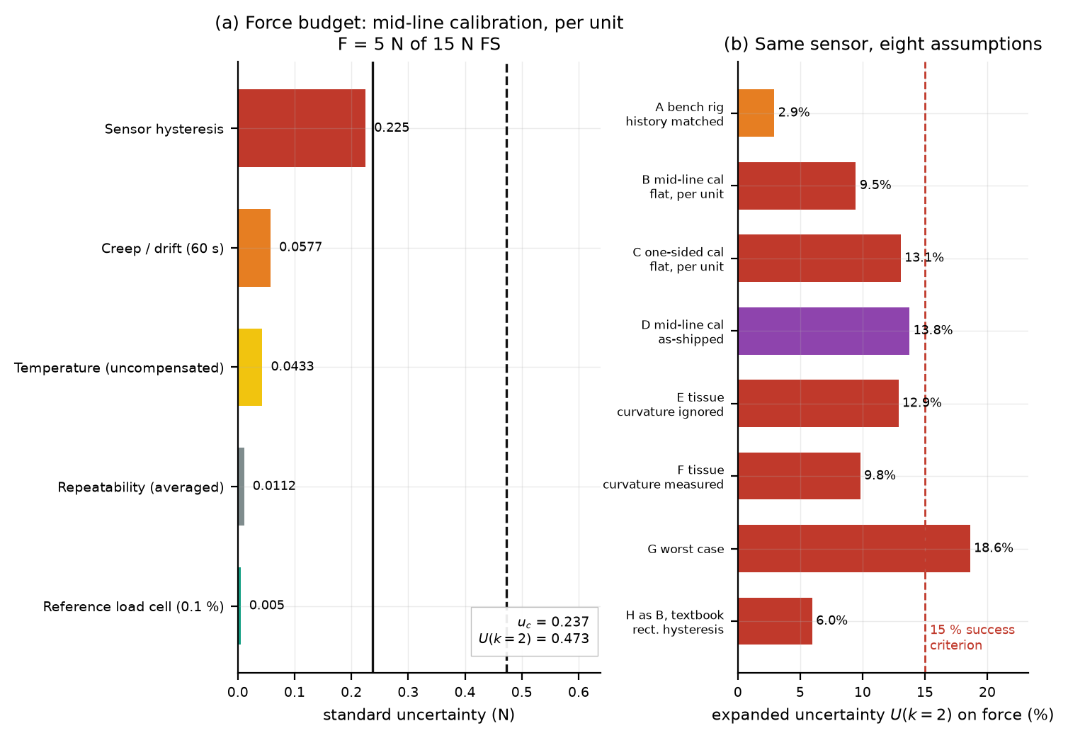
• Absolute force on a geometry-matched phantom: U(k=2) = 9.5 %, 90 % of the variance from hysteresis (results/budget_force.csv, 5 N of 15 N FS). With a matched loading history the same sensor reaches 2.9 % — a factor 3.2 that is protocol, not sensor.
• Stiffness is worse, and contact geometry dominates. U(k=2) on E is 16.4 % with curvature ignored, 14.1 % measured — ±0.82 kPa at 5 kPa, ±3.28 at 20 kPa. Phantom versus 5 mm vessel is a 42 % bias (results/curvature.csv).
• The published 4.2 % is not sample-limited: n_cal 10→50 moves held-out error 4.58→4.69 %. The budget is confirmed to 2 % in the random-branch regime and corrected by 1.6× against the textbook treatment of hysteresis.
• The phantom need not be primary — it must be a 1.4 % artefact. The 1/3 rule demands ≤ 1.50 %; deadweight indentation with a measured Poisson ratio gives 1.42 % for EUR 3,200, against 5.0 % for a EUR 60,000 rheometer.
• The kill criterion is mis-stated; corrected, it is sharper. Hysteresis never kills absolute force at 1–10 %FS (0.955 N of 3σ ambiguity at 3 %FS). What dies is contrast below 19 % at 3 %FS, via h_crit/FS = 0.471·c·(F₀/FS): fat-vs-muscle clears that 15.7×, steatosis I-vs-II fails 2×.

2. What is done, and what is not

Force realisation is not the hard part. NIST deadweight machines realise force at 0.0005 % relative standard uncertainty [1]; force-proving instruments are calibrated under ISO 376 [2] and force-measuring instruments under ASTM E74, though neither standard’s numeric criteria was read. The reference load cell assumed here contributes 0.1 % of reading [ASSUMP] — 200× worse than NIST, and still the smallest term below.

Absolute-newton regression is published. FeelAnyForce reports 4.2 % mean L1 over 0–15 N on unseen objects, 4.8–6.3 % across unseen sensors and gels [3]; DIGIT Pinki reports 5 mN resolution and 3.5–3.9 mN RMSE [4]. Neither reports an expanded uncertainty, or separates repeatability from hysteresis, creep, temperature and gain.

Absolute stiffness calibration is open. No SI-traceable soft-modulus artefact in 1–100 kPa was identified, and no standard for tissue-phantom elastic properties was identified [10, 11] — weaker than “none exists”. Phantoms are characterised by the indenter that later tests the sensor. New here: an uncertainty chain, a simulation that tests it, and a design calculation for how good a phantom must be.

3. Uncertainty budget

3.1 Model

F = (4/3)·E/(1-ν²)·√R·δ^1.5, so E = F(1-ν²)/[(4/3)√R δ^1.5]. Relative sensitivities: 1 on F, 1.5 on δ, 0.5 on R, 2ν/(1-ν²) on ν. Hertz is a consistent propagation model, not a claim about gel physics.

3.2 Hysteresis: model, and why the textbook treatment is wrong

A discrete play (backlash) operator: s ← clip(s + 2ΔF/w, -1, +1), indicated force F + (w/2)s, loop width w = h·FS — reproducing loop width and memory. It saturates, so the residual is binary, one of two points w apart: sd w/2 for a mid-line calibration, not the GUM rectangular w/(2√3). The textbook treatment understates the term by √3 — 6.0 % against a simulated 9.5 %.

3.3 The budget

At F₀ = 5 N of 15 N FS, mid-line, per unit (results/budget_force.csv, variant B):

Hysteresis holds 90 % of the variance, the load cell 0.04 %. Dominant term: hysteresis for force per unit on matched geometry; as shipped, unit-to-unit gain (53 %); on tissue, hysteresis 30 % with contact curvature 28 % close behind.

(a) Per-unit calibration beats any sensor improvement. The gain spread (5 %, 1σ [ASSUMP]) takes U(k=2) to 13.77 %, gain dominant at 53 %; at 15 %, 31 % — the top of the 324-case grid, where U(k=2) spans 3.15–31.1 % (force) and 13.7–38.9 % (stiffness).

(b) The stiffness budget is geometry-dominated (results/budget_stiffness.csv, curvature ignored): hysteresis 4.50 %, contact area/curvature 4.37 %, indentation depth 3.00 %, phantom modulus 3.00 %, Poisson 2.58 %, indenter radius 1.00 %, the rest 1.15/0.87/0.22/0.10 % → combined 8.19 %, expanded 16.38 %. The Poisson term is invisible in the tactile literature: 1-ν² at ν = 0.49 is 0.76, so ±0.02 on ν moves the answer ±2.6 %. Soft-tissue moduli cannot be stated better than ~3 % even with perfect force measurement.

4. Monte Carlo

4.1 Design

mc_calibration simulates 3 phantoms × n_cal ∈ {10…50} per leg × 600 units per cell, fits an affine inverse calibration, and evaluates on a held-out phantom 3× stiffer and a held-out sensor calibrated by transfer. Seed 20261101.

4.2 What it confirms

Four regimes, analytic u_c against MC rms: 4.73/4.66, 6.88/6.77, 6.53/6.50, 8.22/8.11 % — ratios 0.984–0.995 (results/mc_vs_analytic.csv).

4.3 Where it corrects the arithmetic

One-sided calibration with matched loading history gives 0.51 %, not 6.53 % — a ratio of 0.078. The play-operator offset is then a constant the affine fit absorbs, and the mid-line fit shows the same (0.69). Hysteresis is a calibration-history defect, not a sensor defect. Any tactile hysteresis term should be quoted with the loading protocol it was measured under.

4.4 What it condemns

Across n_cal = 10…50 the held-out rms moves 4.58 → 4.69 % (mid-line, random branch) and 7.03 → 7.04 % (as-shipped population); only the matched case converges, by n_cal ≈ 30. A 200,000-indentation training set [3] cannot fix a 4.5 % hysteresis bias: the bias lives in the input space, not the sample. The published 4.2 % and this 4.7 % are the same kind of number, and neither is sample-limited.

Held-out phantom is worse: at 10 % stiffness coupling — a 3× stiffer material shifting the reading 10 %, as an area-only force feature does — unseen-stiffness error is 19.0 % (5 % coupling 10.1 %, 2 % coupling 5.4 %). Held-out-material force error is therefore dominated by an unmeasured property of the regression model.

4.5 Out-of-distribution detection

The claim asks for ≥ 90 % of unseen materials caught (results/ood.csv, Mahalanobis at a 5 % false-positive rate). TPR, 3-D static features versus 4-D with a rate channel: 89.6/86.6 % (100–400 kPa), 100/100 % (1–2 kPa), 6.0/6.4 % (60–80 kPa, just outside the band), 4.7/100 % for identical stiffness at three times the loss tangent. A material just outside the band is caught 6 % of the time, and a loss-tangent change is invisible without a rate channel. The ≥ 90 % claim is a property of the feature set, not the calibration.

5. Phantom design

5.1 The requirement

Against the dominant 4.50 % hysteresis term the 1/3 rule demands ≤ 1.50 %. Inverting is more useful — a worse sensor makes a worse phantom acceptable:

5.2 The three routes

(a) Deadweight indentation. Force is mass × local g, 0.010 % including uncorrected buoyancy — the chain everyone worries about is negligible. Everything is specimen geometry and constitutive assumption: displacement 0.2 %, contact radius 10 µm on 3 mm, finite-thickness model error 1.2 %, and Poisson. With ν assumed it lands at 2.87 % and fails the 1/3 rule by 1.9×; with ν measured (±0.005) it reaches 1.42 %. Recommended.

(b) Rheometer / nanoindenter. Repeatability 1.5 %, better on paper, but a 4 % sampling-volume mismatch is unavoidable (a rheometer shears microlitres; a tactile contact loads cubic millimetres) and the E = 2G(1+ν) conversion re-imports the Poisson problem at 3.4 %. Net 4.99 %, fails; its role is an independent cross-check.

(c) Gravimetric / geometric. Converting density to a modulus needs Flory–Rehner, where χ uncertain at ±0.05 gives 25 % in E — not a modulus realisation at all.

The phantom cannot be made negligible, only adequate: at best 1.42 % against a 4.50 % hysteresis term. Inverted — the phantom is adequate if and only if hysteresis exceeds 2.83 %FS, which is where every real vision-based tactile sensor sits.

6. Resolution versus tissue contrast, and the kill criterion

6.1 The crossover

Classes differing in modulus by c = (E₂-E₁)/E₁ differ in force at fixed indentation by ΔF = c·F₀ (F ∝ E). With hysteresis ambiguity sd u_h per reading, 3√2·u_h < ΔF gives

h_crit/FS = 0.4714 · c · (F₀/FS)     mid-line
h_crit/FS = 0.3333 · c · (F₀/FS)     one-sided

6.2 The numbers

At F₀/FS = 1/3 and h = 3 %FS [ASSUMP], mid-line (results/kill_criterion.csv):

Resolvable contrast floor: 19.1 % at 3 %FS mid-line, 27.0 % one-sided (results/contrast_floor.csv), exactly proportional to h — 6.4 % at 1 %FS, 64 % at 10 %FS.

6.3 Verdict on the kill criterion

The original — “if sensor hysteresis exceeds the tissue differences being resolved, absolute force is not recoverable” — is false as stated and true in a relocated form. False, because absolute force survives even 10 %FS: the 3σ band is 3.2 N there, U(k=2) of 13 % at worst, and under a matched history it cancels entirely (§4.3). True, and worse, for contrast: at 3 %FS nothing closer than 19 % is separable — steatosis grading (10 %) and mild inflammation (15 %) are excluded. The separations the idea names — fat/muscle 200–300 %, artery 100 % — clear the crossover by 5–16×. The kill fires inside tissue classes, not across them.

7. Calibration protocol

Points. 30 per leg, three legs to 0.95 FS, geometrically spaced so the low-force decade is not under-sampled. Calibrate on the branch you will use, or fit the mid-line and pay 9.46 % instead of 2.93 %.

Randomisation, blinding, drift. Randomise phantom order within session, unit order across sessions and point order within each leg, so drift cannot alias onto a phantom. The analyst fitting the map must not see which phantom or unit produced a run — mid-line versus one-sided is a degree of freedom a non-blind analyst can tune. Interleave repeats of the first and last point every 10 min and subtract a per-session linear drift. Hold the enclosure to ±0.2 K — at 0.3 %/K [ASSUMP] a 2 K swing costs 0.87 %.

Acceptance criteria. Lag-1 autocorrelation of residuals below 0.2 — an un-averaged hysteresis loop appears as residual correlation, not scatter; drift-corrected residual sd within 20 % of §3’s prediction; two of three units agreeing on fitted gain within their u_c.

Power. Distinguishing 15 % from 4.2 % [3] is trivial at sample level — n = 3 held-out samples give > 95 % power (results/power.csv), the gap being 10.8 points against ~2.3 of spread. That is not the binding constraint and should not be quoted as if it were. At unit level, paired: sd 4 % gives 0.67 power at 3 units, 0.93 at 4, 0.99 at 5; at 6 %, 0.85 at 5 and 0.94 at 6. Use 5 units, paired.

8. Costs

results/bom.csv: total EUR 3,751, inside the EUR 5,000 ceiling, excluding a shared rheometer. Largest lines: Class F1 weights 640, motorised stage + indicator 480, load cell 420, consumables and moulds 325, indenters 270, granite plate 260, contingency 461. The load cell is the largest scientific line and the smallest uncertainty term. The one uncosted item, a lateral extensometer separating the 2.87 % route from the 1.42 % one, is likely EUR 800–1,500.

9. Limits

Assumptions, not measurements. The structure — hysteresis dominant on force, geometry and Poisson on stiffness, phantom adequate only at 1.4 % — follows from the sensitivities and is robust. The values are only as good as the inputs; the 324-case grid (3.15–31.1 %) is the honest width. No standard is claimed: ISO 376 was seen as a title only and ASTM E74 by name only, and no standard for tissue-phantom elastic properties was identified.

Three weaknesses. (1) Hysteresis, creep and temperature coefficients are unverified: the prior review found no peer-reviewed values for GelSight/DIGIT elastomers, so the 1–10 %FS, 0.5–5 %/60 s and 0.1–1 %/K ranges are the brief’s. One loop on one real sensor — a day’s work — would replace an assumption with a number. (2) Hertz is a placeholder: soft gels are hyperelastic and viscoelastic, so the coefficients would shift without reordering the budget. (3) The OOD simulation models a detector, it is not one.

What would falsify the main claim. A measured hysteresis loop below 1 %FS combined with a matchable use-time history would drop U(k=2) for force to ~2 % and tighten the phantom requirement to 0.6 % — below what route (a) delivers. The chain would then be limited by the artefact, not the sensor, and the project would move from tactile sensing to materials metrology.

Figures

Force uncertainty budget: contributions and the combined standard uncertainty.

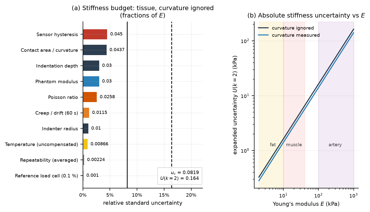
Stiffness uncertainty budget — contact geometry and Poisson ratio, not force.

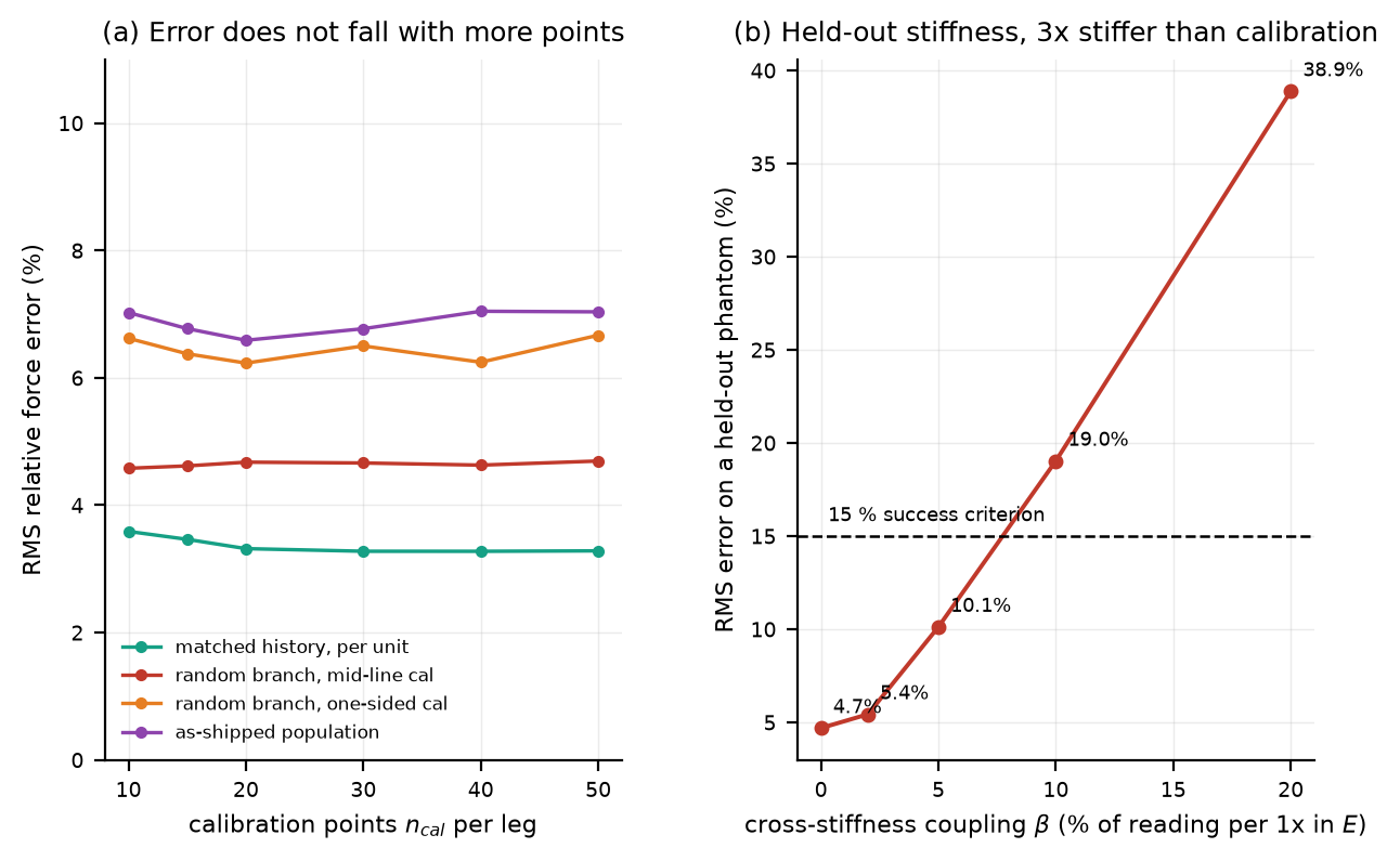
Monte Carlo against the analytic budget; the two agree to 2 % after the play-operator correction.

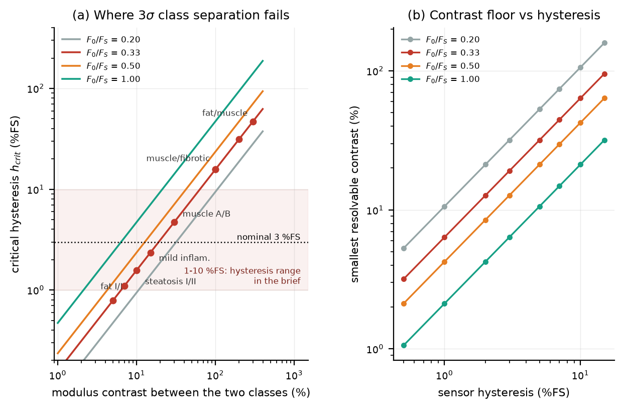
The corrected kill criterion: resolvable contrast against hysteresis and operating point.

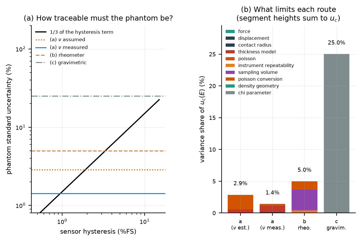
Phantom realisation routes against the 1/3 rule: deadweight with measured Poisson ratio is the only one that passes.

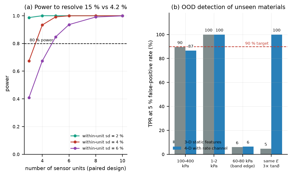
Power for the paired unit-level design and out-of-distribution detection performance.