H0346 — Hydrogel skin perforation: a 2-D axisymmetric transport dossier

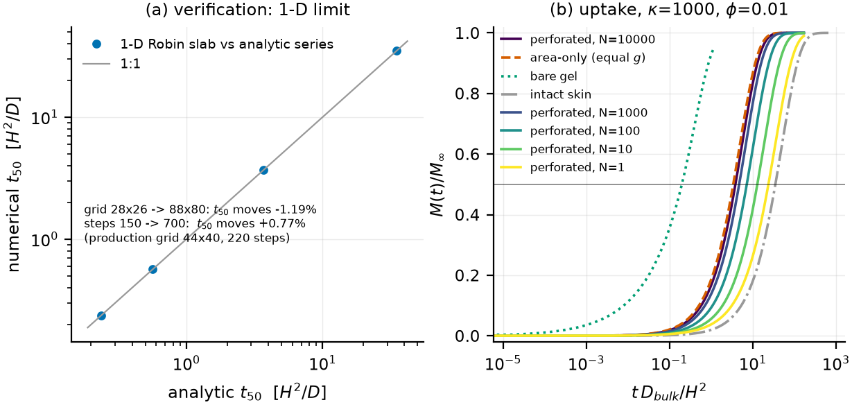
Status: model only. No experimental data were generated or used. Every number below is produced by code/diffusion2d.py, code/analysis_figures.py and code/power_bom.py and is stored in results/; the file each number comes from is named in the text. Times are quoted dimensionlessly as $t\,D_{bulk}/H^2$ and, where useful, in hours using the stated modelling assumption $D_{bulk}=10^{-10}\,\mathrm{m^2\,s^{-1}}$, $H=1$ mm (so $t[\mathrm{s}] = 10^4\,t^*$).

Summary

• The claim fails in all 208 layouts computed. The gain factor against a properly constructed area-only control is $G_K \in [0.084,\,0.961]$, median 0.595; it never exceeds 1 in a single case (results/summary.json, results/derived.json). Perforations always deliver less than their open area’s worth of conductance — shadowing beats funneling everywhere in the explored space.
• The deficit is governed by $a/\delta$, the hole radius divided by the skin thickness — not by the open-area fraction $\phi$. Across all 208 layouts (κ = 10…10⁴, φ = 2.5×10⁻⁴…0.5, δ/H = 0.01…0.1) the gain collapses onto $G_K \approx 1/(1+0.45\,(a/\delta)^{0.84})$ (prefactor 0.453, exponent 0.842, r = 0.898 over 208 points; results/derived.json: X_fit_all; Fig. 3a).
• At fixed open area, hole size changes the answer by 6.5×. For κ = 1000, φ = 0.01: one 1 mm hole gives $t_{50}=23.86$, 30 000 holes of 6 µm give $t_{50}=3.66$ (results/sweepA_phi_N.csv). The brief’s “sparse perforations” is precisely the worst configuration available.
• The apparent “disproportionate gain” is a path-length artefact, and it is large: $G_0 = K_{perf}/(\phi K_{bare})$ ranges 1.9–504, median 13.5. It appears only because a 50 µm bore is compared with a 1 mm gel path. It contains no information about the hole’s footprint (Fig. 5).
• A decisive experiment is cheap and does not need a sub-5 µm thinned-skin control: hold φ fixed and vary hole size, or hold hole size fixed and vary spacing. A bench realisation is costed at EUR 2 551 (results/bom.csv), within the EUR 3 000 ceiling.

1. The claim

The incoprea catalogue (ID H0346) asserts:

A dense skin layer forms on a hydrogel; sparse perforations in that skin will reduce the swelling delay more than their fractional open area would predict.

Primary outcome: time to half of equilibrium swelling, $t_{50}$, at the same final swelling ratio. Kill criterion: if an area-only transport model explains the result, the disproportionate-gain claim is rejected.

The scientific problem is that “fractional open area would predict” is not one model but at least three, and they differ by two orders of magnitude. Fixing the baseline is the whole analysis, so §3 states all of them explicitly.

2. Model

Geometry. A gel disc of radius $R = 10$ mm and thickness $H = 1$ mm with a dense skin of thickness $\delta = 50$ µm on the top face and an impermeable support at the bottom. Skin diffusivity is $D_{skin}=D_{bulk}/\kappa$.

Reduction. The hexagonal array is periodic and its Voronoi cell has zero normal flux on its faces, so we solve one cell as an axisymmetric cylinder of radius $R_{cell}=R/\sqrt{N}$ (equal areas), replacing the hexagon by an equal-area circle. Then $s=R\sqrt{2\pi/(\sqrt3 N)}$ is the nearest-neighbour spacing, $a=R\sqrt{\phi/N}$ the hole radius, $\phi=a^2/R_{cell}^2$. The geometry depends only on $(a,\phi)$; $R$ sets how many holes fit.

Equation and boundary conditions. Dimensionless with lengths by $H$, time by $H^2/D_{bulk}$, concentration by $c_{eq}$:

$$\frac{\partial c}{\partial t}=\frac1r\frac{\partial}{\partial r}\left(rD\frac{\partial c}{\partial r}\right)+\frac{\partial}{\partial z}\left(D\frac{\partial c}{\partial z}\right),\qquad -D\frac{\partial c}{\partial z}\bigg|_{z=1}=h(r)\,(1-c)$$

with no flux at $z=0$, symmetry at $r=0$, no flux at $r=R_{cell}$ (the periodic neighbour), and $h_{skin}=1/(\kappa\delta/H)$ over the skin, $h_{hole}=H/\delta$ over a bore ($r<a$) — the brief’s own definition “$D=D_{bulk}$ at the surface”. The gel-side spreading resistance is not put in by hand; the solver computes it. An earlier version also added the classical $1/(4Da)$ access resistance to $h_{hole}$ and double-counted it, inflating the total resistance by ~35 %.

Discretisation. Cell-centred finite volume in $(r,z)$, harmonic-mean face conductivities, grids graded on the hole rim and the top surface, boundary conductances referred to the cell centre (with the half-cell series term, else the permeance is biased by $O(\Delta z)$), implicit Euler with geometrically growing steps, per-layout time windows sized from the analytic 1-D slab solution so that fast layouts are not integrated more coarsely than their own $t_{50}$.

Baselines. Three, all evaluated with the same solver on the same mesh:

B1 and B2 coincide at the nominal $r_w=1$. B2 is the only rule-of-mixtures model that is a fair area-only control for the same hole: it credits the hole with exactly the conductance the hole has, then asks whether concentrating that conductance in φ of the area beats spreading it out.

The uniformly thinned skin is identical to B1/B2, not a separate control: equal sheet conductance requires $\delta_{thin}=\delta/(\phi\kappa+1-\phi)$ = 4.55 µm at the nominal parameters, not the naive $\delta(1-\phi)=49.5$ µm, whose conductance is only 1.01× the intact skin and is therefore not transport-equivalent at all (results/sweepA_phi_N.csv).

Metric. $G_K=(K_{perf}-K_{intact})/(K_{area}-K_{intact})$ for the steady permeation conductance (reservoir on top, perfect sink at the bottom) and $G_t=(1/t_{50,perf}-1/t_{50,intact})/(1/t_{50,area}-1/t_{50,intact})$ for the kinetics. $G=1$ means exactly area-proportional; $G>1$ is the claim.

Verification (results/validation.csv, Fig. 1a): against the analytic Robin-slab series, $t_{50}$ within 0.47 % and $\max|M/M_\infty-M_{exact}|=0.0036$ over Bi = 0.02…20; grid 28×26 → 88×80 moves $t_{50}$ by 1.19 % and 150 → 700 steps by 0.77 % (production: 44×40, 220 steps); a Dirichlet patch on a half-space reproduces the classical $4Da$ access conductance to −8.1 % … +0.97 %, the limit being the integrable rim singularity; and the lumped Robin skin agrees with a fully resolved skin slab plus a real bore to 0.4–1.6 % in permeance, which licenses the lumped treatment.

3. Results

Nominal case (κ = 1000, φ = 0.01, δ/H = 0.05, N = 100, a = 100 µm, s = 1.90 mm; results/derived.json: nominal):

The perforation buys a real 4.87× speed-up, but the area-only model predicts 10.3×: $G_K = 0.444$, $G_t = 0.416$ — the perforation delivers 42–44 % of what its open area promises.

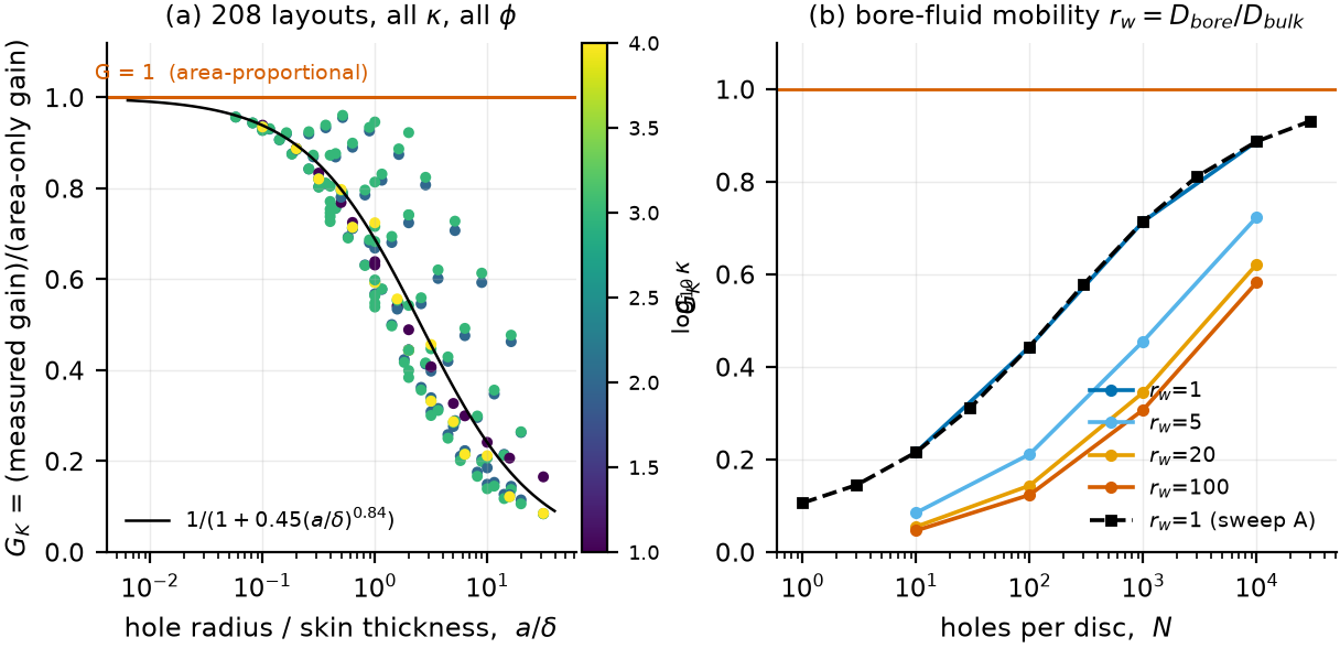
The gain map. Over all 208 layouts, $G_K$ never reaches 1 (results/summary.json: min 0.084, max 0.961, median 0.595, fraction > 1 = 0.0). $G_t$ is slightly harsher (min 0.051, max 0.956, median 0.556). The extreme cases are informative:

• Worst: $G_K = 0.084$ at κ = 1000, φ = 0.01, N = 10, δ/H = 0.01 (a = 316 µm, s = 6.0 mm): $t_{50}$ falls only 7.21 → 5.11 where the area-only model says 0.86. One hole every 6 mm is not a perforation, it is a defect. Worst kinetics: $G_t = 0.051$ at N = 1 ($t_{50}=23.86$ vs 3.41) — a single hole in a 20 mm disc recovers almost nothing.
• Best: $G_K = 0.961$ at φ = 0.2, N = 30 000, a = 25.8 µm — an 82.8× speed-up, essentially at the area-only limit but still not past it.

$G_K$ collapses onto a single function of $a/\delta$ (Fig. 3a), fitted as $G_K = 1/(1+0.453\,(a/\delta)^{0.842})$ with r = 0.898 on log-log axes over 208 points (results/derived.json: X_fit_all). The scatter in the prefactor is roughly a factor of two (the ratio $X/(a/\delta)$, with $X=1/G_K-1$, has median 0.51 and IQR 0.26–0.67 in sweep A), so the relation is a scaling law, not a precise formula. The dependence on κ is weak once κ ≥ 100 and the dependence on φ is weak at fixed $a/\delta$; what matters is the ratio of the hole radius to the skin thickness.

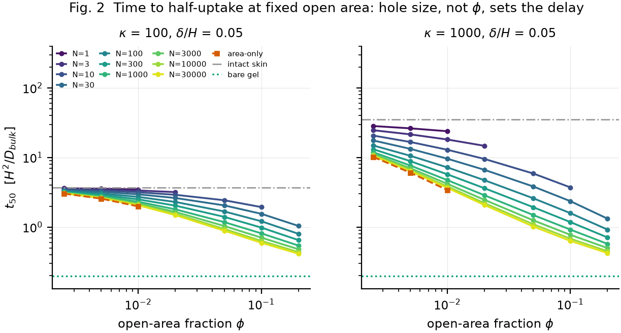
Hole size at fixed open area (Fig. 2, results/sweepA_phi_N.csv). At κ = 1000, φ = 0.01, $t_{50}$ ranges from 23.86 (N = 1) to 3.66 (N = 30 000) — a 6.5× span at identical open area, identical final uptake and identical skin. This is the single most important number in the dossier: the open-area fraction is not a predictive variable; the hole size is.

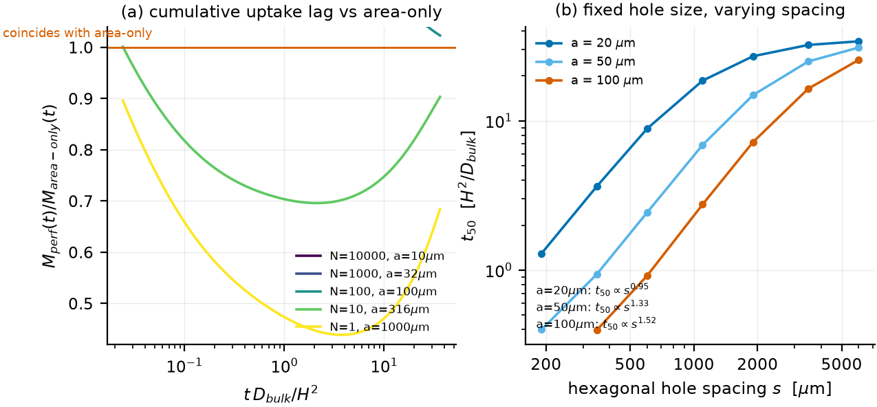
Spacing at fixed hole size (Fig. 4b, results/sweepC_spacing.csv). $t_{50}$ falls as a power of spacing but the exponent is sub-quadratic: 0.95 (a = 20 µm), 1.33 (50 µm), 1.52 (100 µm) (results/derived.json: spacing_scaling). At fixed $a$ the open fraction rises quadratically, and beyond φ ≈ 0.05 the gel’s internal diffusion resistance becomes co-limiting, so further holes stop buying time — the same saturation that caps the area-only model.

Bore-fluid mobility (Fig. 3b, results/sweepE_bore_fluid.csv). A more conductive bore ($r_w>1$) makes the deficit worse, not better — at N = 100, $G_K$ = 0.444 ($r_w$=1), 0.211 (5), 0.144 (20), 0.124 (100) — because the bottleneck moves into the gel beneath the hole, where a 100 µm patch must feed a 1 mm-deep cell.

Skin thickness and κ (results/sweepB_beta_kappa.csv). At κ = 1000, N = 100: $G_K$ = 0.21, 0.29, 0.44, 0.59 for δ/H = 0.01, 0.02, 0.05, 0.10. Thicker skins are closer to area-proportional because the bore resistance $\delta/(\pi a^2 D)$ then dominates the access resistance. κ matters only below ~100: at N = 100, $G_K$ = 0.49 (κ=10), 0.44 (κ=100), 0.44 (κ=1000), 0.44 (κ=10 000).

4. Where the claim survives, and where it dies

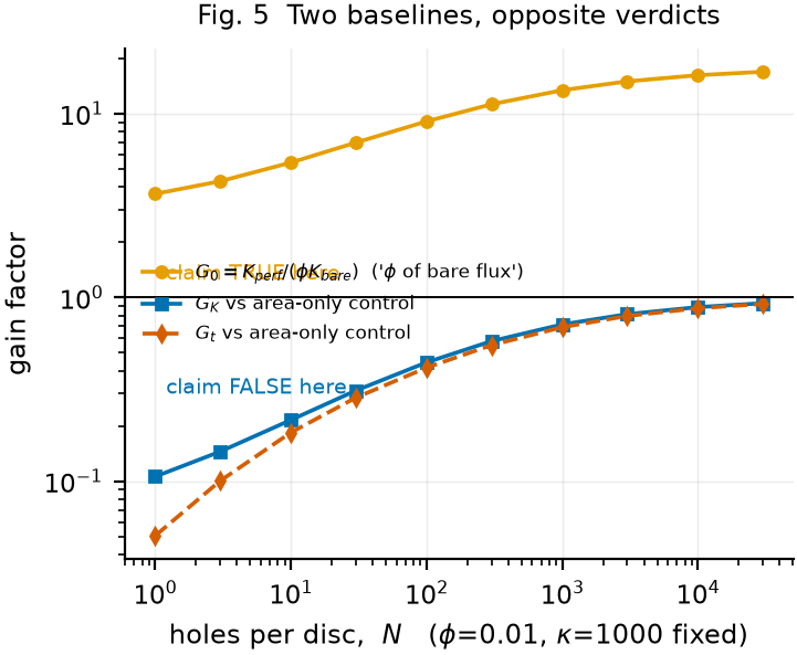
It survives, and looks spectacular, against B0. $G_0=K_{perf}/(\phi K_{bare})$ ranges 1.9–504, median 13.5 (Fig. 5): at the nominal case a 1 % perforation delivers 9.1× the flux that 1 % of bare gel would. Read as “1 % open area buys 900 % of the bare flux” the hypothesis looks confirmed by an order of magnitude. This is, I believe, where it came from.

It dies against B1/B2, and the reason is exact without the solver. A bore of radius $a$ and depth $\delta$ must, besides its channel resistance $\delta/(\pi a^2 D)$, push its flux into the gel through a constriction of resistance $\sim 1/(4Da)$; the ratio of the two is $\pi a/(4\delta)$. The area-only model keeps the first term and drops the second. Since $\delta \ll H$ and no manufacturable layout has $a < \delta$, the dropped term dominates and $G<1$ follows. The solver reproduces the scaling of that dropped term without being told about it: fitted exponent 0.84 on $a/\delta$, prefactor 0.45 ≈ $\pi/4\cdot 0.6$.

Closest to true — the only window worth an experiment: $a/\delta \lesssim 0.3$ with dense packing (a few µm holes in a 50 µm skin, $N \gtrsim 10^4$ per 20 mm disc), where $G_K = 0.887$–0.961 and the 82.8× speed-up is genuine. Even there the gain is not disproportionate; it is area-proportional and simply no longer access-limited.

Fails hardest for sparse, large holes: $a/\delta \gtrsim 5$ gives $G_K \lesssim 0.25$, and $N=1$–10 gives $G_t \approx 0.05$–0.2 — precisely the proposed configuration.

5. Experimental realisation

Specimens. PVA (99+ % hydrolysed, 10 wt %) cast in 10 mm silicone wells, freeze–thawed 3× (−20/+20 °C, 6 h each); a dense skin by controlled drying of the top face at 45 °C — so skin thickness is a process variable to be measured, not assumed. Holes by 405 nm diode laser on an XY stage (a = 20–200 µm) or pin gauges (a ≥ 100 µm): two routes, because laser drilling of 20 µm holes in a 50 µm skin is the risky one.

Measurement. Mass uptake on a 0.1 mg balance, ~20 points per specimen, blotting standardised to 2 s, 25.0 ± 0.1 °C. Controls in order of importance: (1) open area measured optically, not assumed — it is the x-axis of the claim and the likeliest source of a false positive; (2) hole edges inspected at 200× (a melted rim is a larger hole); (3) $H$ and $\delta$ per specimen, since $a/\delta$ is the controlling variable; (4) final uptake must match across layouts, the cheap check on “same final swelling ratio”; (5) a bare-gel arm, which fixes $D_{bulk}$ and converts $t_{50}^*$ to seconds.

Sample size. For a two-group comparison at α = 0.05, power 0.80, a 20 % difference in $t_{50}$ and CV = 5, 7.5, 10 %, the requirement is 3, 3, 4 specimens per arm (results/power.csv: two_group_t). But $G$ is a ratio of differences, so its error is amplified: a Monte-Carlo over the estimator at the nominal model values (G = 0.416) gives a 95 % CI width on $G$ of 0.083 (n = 5, CV = 7.5 %) and 0.112 (n = 5, CV = 10 %), i.e. ±10–13 % relative (results/power.csv: MC_estimator_G). Power to reject $G \ge 1$ is 1.00 at every n ≥ 3 in that Monte-Carlo, because the model puts $G$ at 0.42, not at 0.9. Plan for n = 6 per arm, which absorbs batch-to-batch variation in $\delta$ that the within-batch CV does not capture.

The decisive, low-risk experiment. Do not try to fabricate the 4.55 µm thinned-skin control — it is not manufacturable repeatably, and the model says the control is indistinguishable from the area-only calculation anyway. Instead hold φ = 0.01 fixed and make three perforated plates with a = 32, 100, 316 µm (N = 1 000, 100, 10). The model predicts $t_{50}$ = 4.73, 7.21, 12.92 in units of $H^2/D$ (results/sweepA_phi_N.csv, κ = 1000 rows) — a 2.7× span at identical open area. A monotone dependence on hole size at constant open area is the refutation of the claim, and it needs no thinned-skin specimen at all.

6. Costs

EUR 2 551 (results/bom.csv), ex-VAT, indicative catalogue prices — no quotations were obtained. The three items that dominate are the 0.1 mg balance (EUR 620), the convection oven (EUR 480) and the laser module with stage (EUR 420). The items that make the result interpretable rather than merely reproducible are the USB microscope (EUR 145, for the optically measured open area) and the micrometer (EUR 130, for $\delta$). A laboratory that already owns a balance and an oven can run this for about EUR 1 000. There is no item on the list that is not needed; the ceiling is not the binding constraint, the laser drilling of 20 µm holes in a 50 µm skin is.

7. What would falsify this

The distinctive prediction is not “$G<1$” — that is only directional. It is the scaling:

1. $t_{50}$ at fixed φ must rise strongly with hole size, roughly as $1+0.45(a/\delta)^{0.84}$. Three hole sizes at constant open area showing no hole-size dependence would kill the Fickian constriction picture and put the claim back in play.
2. $G$ must depend on $a/\delta$ and be nearly φ-independent at fixed $a/\delta$; a measured φ-dependence falsifies the collapse of Fig. 3a.
3. Any layout with $G_K>1$ and a CI excluding 1 falsifies this dossier outright.
4. $t_{50}\propto H^2$. An exponent near 1 (poroelastic, surface-limited) invalidates the diffusion framing and with it both the claim and this refutation.

8. Limits of the model

• 2-D axisymmetry, equal-area circular unit cell. The hexagonal Voronoi cell becomes a circle of the same area (error largest when $a/R_{cell}$ is not small; unquantified). The model is an infinite periodic array: the rim of a real disc is absent, so a specimen with holes to the edge will be slightly faster than predicted — a bias against this dossier’s own conclusion.
• Fickian, linear, constant $D$; no case-II front, no moving boundary, no gel expansion, so the skin is never stretched and never cracks. Real skins craze, and a craze is an unplanned perforation: again a bias against the conclusion.
• No poroelastic coupling. The Tanaka / Hong–Zhao–Suo framework (prior-art §4, refs [13],[14],[15]) is not implemented; this is the linearised, small-strain limit, and a poroelastic gel could show a qualitatively different $t_{50}$–thickness relation.
• No skin swelling or capacity. The skin is a pure barrier; its water capacity is $O(\delta/H)=5$ %, bounding that approximation, but a skin that thins as it swells would change $\delta$ during the run.
• $D_{bulk}$ and $D_{bore}$ are assumptions, not measurements. The prior-art file is explicit (§7) that no verified cooperative-diffusion value was available; the $10^{-10}$ m² s⁻¹ used here is a modelling choice, and all times scale as $1/D_{bulk}$. The ratios that decide the verdict ($a/\delta$, $G$) do not depend on it.
• The bore model is the weakest assumption. $r_w = D_{bore}/D_{bulk}$ is set to 1 (the brief’s definition). The sensitivity sweep shows that a water-filled bore ($r_w = 20$) makes the deficit roughly three times worse (results/sweepE_bore_fluid.csv), so the nominal is the most favourable case for the claim; no plausible $r_w$ reverses the sign.

Provenance

code/diffusion2d.py (solver, validation, sweeps; deterministic, 141 s wall) code/analysis_figures.py (fits, results/derived.json, figures) code/power_bom.py (power calculation, BOM) Results: sweepA_phi_N.csv (124 layouts), sweepB_beta_kappa.csv (64), sweepC_spacing.csv (20), sweepD_gain_curves.csv (time-resolved), sweepE_bore_fluid.csv (16), validation.csv, power.csv, bom.csv, summary.json, derived.json.

Figures