A magnetic smoke alarm for batteries: a sensitivity link budget

Direction 05-13, from incoprea.com Frontier Idea #13. Every number below is produced by code/magnetostatics.py and is traceable to a named file in results/. Sensor sensitivities are published specifications; every field value is a calculation. No measurement is reported anywhere in this dossier.

1. Summary

• The filament field is small but not absurd: 0.48 nT at 3 mm standoff for a 10 mA filament 1 mm deep, falling as 1/r² to 8.0 pT at 30 mm (filament_field.csv, model element). If the fault current also closes through pack wiring the same 10 mA gives 199 nT at 3 mm and 78 nT at 30 mm (external_loop). That factor of 400 is the largest uncertainty in the idea, and it is a property of the return path, not the sensor.
• Sensor noise is never the binding constraint. An OPM (15 fT/√Hz) sees the 10 mA filament at 3 mm with SNR 3.2 × 10⁴ in 1 Hz; SNR 5 is reached in 1.2 × 10⁻⁸ s (snr_integration.csv). The equivalent detectable current is 1.6 µA.
• The binding constraint is the terminal-current background. 5 A of charging current gives 87 nT at 3 mm modelled as 32 parallel electrode pairs, 2.78 µT as a single pair, and 30.4 µT with opposite-end tabs (background_field.csv). Required common-mode rejection: R = 181 to 5.8 × 10³ (element-only filament), or 0.44 to 153 (external-loop filament).
• Gradiometry works only with a short baseline. A vertical gradiometer with b = 1 mm cuts the required rejection from 181 to 3.9 against the 32-layer background, because the filament is compact and the background is cell-scale. The optimum is b ≲ h; longer baselines are worse (R = 21 at 10 mm, 165 at 100 mm; gradiometer_budget.csv). The balance needed is ε = 4.0 × 10⁻⁴, at the edge of the state of the art.
• Packaging is not the constraint; the 10-minute target is set by chemistry. The 100 µm Al pouch attenuates a quasi-static field by 0.001 dB at 100 Hz, 5.1 dB at 10 kHz (−3 dB at 6.7 kHz; skin_depth.csv); at DC, not at all. For warning time t = τ ln(I_crit/I_detect): a 5.8 × 10³× better threshold moves the required growth constant only from 86 s to 38 s (warning_budget.csv). Sensitivity enters logarithmically, τ linearly; a 10-minute warning needs τ ≳ 85 s.

2. The idea, and what is already published

A lithium filament concentrates current before it shorts; an NV-diamond or OPM magnetometer outside the pouch might see the resulting field early enough to warn before voltage collapse. The original decisive test was median warning > 10 min with < 1 false positive per 100 cycles.

The prior-art review (_lit/A_battery_prior_art.md) supplies what this dossier does not redo. Magnetic sensing of cells is an established diagnostic field: Bason et al. (J. Power Sources 2022) imaged a pouch cell’s internal current distribution while cycling and resolved percent-level deviations; Evans et al. (arXiv:2512.01125, 2025) measured 500 fT relaxation features on 6000 mAh cells with a QuSpin-class OPM array at < 1 cm standoff, benchmarked against a 304-channel SQUID at 50 mm, 3 fT/√Hz; Chen et al. (Materials 15, 1980, 2022) built a 16-channel magnetoelectric array at 3–5 pT/√Hz at 10 Hz. The widely quoted “magnetics leads temperature by 100×” is a simulation (Bai et al., Sci. Rep. 14, 2024), and the closest claim to magnetic plating detection (Qi et al., IET Conf. Proc. 2025) is explicitly “verified through simulation”. Decisively, no one has published a quantified “how small a filament can be seen at what standoff with what averaging time” link budget: Liang et al. (J. Phys. Energy 8, 032003, 2026) list metal casings, eddy currents and stack-level backgrounds as unresolved, and the prior-art review reports zero occurrences of “gradiometer” in that 26-page document. That gap is what this dossier fills.

3. Forward model

Geometry (summary.json → assumptions): 150 × 90 × 10 mm stack, sensors at z = +5 mm + h. Al laminate 100 µm, Al collector 15 µm, Cu collector 10 µm, separator 20 µm, μ_r = 1, charging current 5 A (≈1C for 5 Ah).

Method. Each distribution is discretised into elements carrying a moment m = J dV or K dA, and the field is the exact superposition B = (μ₀/4π) Σ m × (r−rᵢ)/|r−rᵢ|³. Distributions conserve charge by construction: the terminal current is a hairpin with lateral collector current tapering linearly from I_ch at the tab to zero at the far edge, and uniform through-stack density j_z = I_ch/(LW) between the collectors.

Validation (validation.json) against three analytic limits:

Sheet and wire residuals are finite-size truncation, not discretisation. Grid convergence at 3 mm: 2.663 / 2.784 / 2.785 µT at 3 / 1.5 / 1.0 mm voxels (0.01 % between the last two), so 1.5 mm voxels are used.

Two results contradict the natural first guess.

(a) The field of the filament element on its own axis is exactly zero — Biot–Savart gives dl × r̂ = 0 there, so a sensor directly above the fault sees nothing from the element. The field appears off-axis, peaking at ρ ≈ h + depth. Every field here is a peak over a 40 × 40 mm sensor window; the B_onaxis_nT column of filament_field.csv is identically zero to make the point.

(b) A purely radial-plus-axial return current produces no axial field either. The fault loop (up the filament, out along the electrode plane, back through the terminal) has no azimuthal element, so its B_z on axis vanishes identically: symmetric_radial_return_on_axis returns 7 × 10⁻¹⁹ nT for a 45 mm radial return carrying 10 mA. The observable is the in-plane field, which is what OPM arrays in fact measure.

Filament radius is irrelevant above r_f. By Ampère the field outside an axially uniform current cylinder is exactly the line-current field, so 10 µm and 200 µm filaments carrying the same current are indistinguishable at any standoff > r_f. Only in contact does radius matter, where B = μ₀I/2πr_f gives 200 µT at 10 µm — the NV regime, which is unreachable through a sealed pouch.

4. Results

4.1 Filament field versus standoff

Peak |B| over the sensor window, 10 mA, 1 mm deep (filament_field.csv):

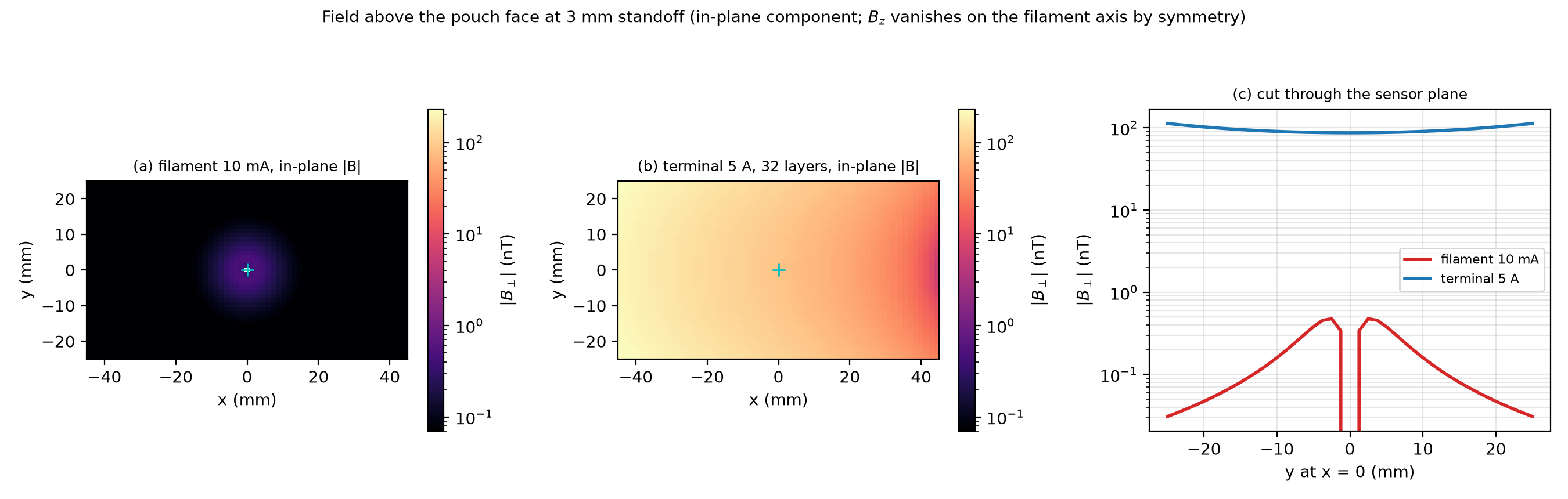
The element model falls as 1/r²; the loop model is nearly flat to 10 mm because the loop is larger than the standoff. No published measurement distinguishes the two, and feasibility turns on which is real. fig1_field_maps.png shows the contrast — a compact blob against a smooth field 180× larger — and fig2_standoff.png plots both branches against the background bands.

4.2 The terminal-current background

This is the most important structural result in the forward model. A real cell is a series of parallel electrode pairs, each carrying I_ch/N, whose collectors carry opposite lateral currents ~0.15 mm apart. That pairing cancels the external field by roughly 1/N², so the naive single-sheet estimate (17.5 µT) is one to two orders too pessimistic. The background is consequently not knowable a priori to better than a factor of ~300, which is why the decisive experiment must measure it.

4.3 Gradiometric contrast — the key number

Vertical gradiometer, 3 mm standoff, 10 mA element (gradiometer_budget.csv):

What baseline and balance are required? The differential signal saturates once b ≳ h + depth while the differential background keeps growing linearly in b, so the optimum is the shortest baseline, b ≈ 1 mm: it buys a factor of 46 in rejection (R falls from 181 for a single sensor to 3.9). Longer baselines actively hurt — at b = 100 mm the gradiometer is no better than a single sensor. The balance required is 4 × 10⁻⁴ against the 32-layer background, 1.3 × 10⁻⁵ against the single-layer background, and 1.2 × 10⁻⁶ against opposite-end tabs. Laboratory first-order gradiometers achieve 10⁻³ to 10⁻⁴, so only the most favourable background model is comfortably in reach (fig3_gradiometer.png).

For the external-loop filament the picture inverts: once the loop contributes 199 nT the signal dominates the background (R = 0.44) and no rejection is needed at all.

5. The binding constraint

Three candidates were tested; one survives.

Packaging — ruled out. skin_depth.csv: δ(Al) runs from 81.9 mm at 1 Hz to 0.259 mm at 100 kHz. The thin-slab transmission |1 + jωτ|⁻¹ with τ = μ₀σtl/2, l = 10 mm, gives 0.001 dB (0.01 %) at 100 Hz, 0.095 dB at 1 kHz, 5.1 dB at 10 kHz, 23.5 dB at 100 kHz; −3 dB falls at 6.7 kHz for Al and 1.4 kHz for Cu. At DC and at any plausible charging ripple the pouch is transparent (fig4_eddy.png), agreeing with the prior-art assessment.

Sensor noise — ruled out. SNR 3.2 × 10⁴ (OPM) and 1.6 × 10⁵ (SQUID) in 1 Hz; time to SNR 5 is 1.2 × 10⁻⁸ s. Even a $500 fluxgate at 10 pT/√Hz sees SNR 48 in 1 s. A 1000× better sensor changes nothing.

Background rejection — this is the binding constraint. The requirement is R = 181 to 5.8 × 10³ (element filament) or 0.44 to 153 (external loop); the achievable rate is set by sensor balance and by how well the current distribution can be modelled. Model-based subtraction does not rescue the unfavourable case: the filament is a percent-level deviation of the current distribution, so a background model good to the percent level — the state of the art per Bason et al. — leaves a residual the same size as the signal it is meant to expose. The rejection must be geometric, and geometry only helps because the filament is compact while the background is extended.

decision_table.csv makes the consequence explicit. With noise alone, the maximum standoff for a 10 mA filament is 100 mm (OPM, 1 s), > 200 mm (SQUID), 30 mm (NV), 15 mm (magnetoelectric), 10 mm (fluxgate). Add the 32-layer background at ε = 10⁻³ and every sensor class collapses to the same 3 mm; at ε = 10⁻⁴ it is 10 mm for every class. Against the single-layer background at ε = 10⁻³ nothing works at any standoff; at ε = 10⁻⁴ the limit is 0.5 mm, i.e. the sensor must touch the pouch. One standoff limit across four sensor classes spanning four orders of sensitivity is the cleanest statement that the sensor is not what is being tested (fig6_decision.png).

6. Warning-time analysis

Detecting a filament and detecting it early are different questions; the second needs an evolution model. Assume exponential growth I_f(t) = I₀ exp(t/τ) up to a collapse current I_crit; then t_warn = τ ln(I_crit/I_detect), independent of I₀. Take I_crit = 10 A (a 0.1 V drop through 10 mΩ, about where a BMS sees the fault) and scan τ over 1–100 s (warning_time.csv, fig5_warning.png). Coupling to the link budget at 3 mm with an OPM (warning_budget.csv):

The warning time is dominated by τ, not by sensitivity: a 5.8 × 10³× improvement in I_detect moves the required τ only from 86 s to 38 s, because the dependence is logarithmic. In the last row the “detected” current is 3.2 A — not a filament but a hard short — so that case is failed, not marginal. The 10-minute target is reachable only if the pre-failure growth is slow, τ ≳ 85 s. No published measurement of τ for a lithium filament in a pouch cell was found in the prior-art review; that assumption, not the magnetometer, carries the 10-minute claim.

7. Decisive experiment

One free parameter dominates — the return-path geometry, worth a factor of 400 in signal. The test needs no lithium and no cell.

Phantom. A pouch-sized Al-laminate envelope (150 × 90 × 10 mm) filled with electrolyte-soaked separator, with a 25 µm Cu wire threaded normal to the face at known position and depth, driven by a floating current source at 1/10/100 mA. A separate tab pair carries the “terminal” current at 0/1/5 A.

Instrumentation. One OPM or a three-axis fluxgate on a manual 3-axis stage at 1/3/10/30 mm standoff in a quiet room. Drive the filament at 1.0 Hz square wave and lock in: that removes 1/f drift and makes the amplitude question trivial.

Four conditions. (1) Terminal current on, filament off — measures the background and its spatial structure; tests the layered-hairpin prediction (87 nT vs 2.78 µT, a factor 32 any magnetometer resolves). (2) Filament on, terminal off — measures the filament field and hence the return-path geometry; prediction 0.48 nT (element) vs 199 nT (loop) at 3 mm, a factor 400. (3) Both on — tests superposition. (4) Repeat (2) with the tabs shorted versus open: this changes the return path directly and should move the signal between the two limits.

Control against the terminal-current background. The 1 Hz modulation is primary: a DC terminal current has no 1 Hz component, so lock-in rejects it by the instrument’s dynamic reserve (> 100 dB). Secondary: condition (1) subtracted from condition (3) at the same terminal current. A null in condition (2) at 3 mm — below 0.1 nT for 10 mA — would kill the element-only model.

Cost. Fluxgate, stage, current source and phantom: ≈ $6–9 k plus about two weeks of one person, borrowing an OPM for the 0.48 nT branch. Buying an OPM (QuSpin QZFM class, ≈ $10–15 k) makes the total ≈ $20–25 k — two to three orders cheaper than a cell-level plating campaign, and it yields the one number the idea depends on.

8. Limits

• The return-path geometry is not derived from first principles. The two limits bracket the answer; neither comes from the electrochemistry of a real soft short. The radial return in the electrode planes is argued to cancel (§3b) but not simulated with a realistic conductivity distribution — that needs a transmission-line model of the electrode pair to fix the current-spreading length λ.
• The background model is an idealisation. Perfectly parallel, identical pairs maximise cancellation; real cells have uneven tab welds, jelly-roll asymmetry and busbar geometry that will raise the background above the 32-layer value. The true level probably lies between the 4-layer (696 nT) and 32-layer (87 nT) rows — a judgement, not a result.
• The NV specification is soft. The brief quotes ~1 pT/√Hz at 10–50 µm; the prior-art review’s own NV numbers are 2 µT/√Hz (CW-ODMR) and 50 nT in 1 s (pulsed). 1 pT/√Hz is used here only as a generous bound. NV is excluded on geometry in any case: a 50 µm standoff is inside the 100 µm laminate.
• τ, I_crit and the exponential law are assumed. All three set the warning time and none is measured; a filament growing by electrodeposition may grow linearly in radius with an accelerating rather than exponential current.
• False-positive rate is not computed. The < 1-in-100-cycles target needs a noise and drift model over months, including sensor temperature coefficient and sub-0.1 Hz drift; only single-shot detectability is computed here.
• Two approximations are unquantified. The tab-return geometry was dropped because its peak is simply the sensor sitting next to the terminal hardware — a pack-layout question. The eddy-current treatment is a thin-slab approximation with a single spatial scale l = 10 mm, ignoring the layered collector stack and finite cell size, so the quoted attenuations are indicative to perhaps a factor of two.

Verdict. The idea is not killed by sensor physics, packaging, or averaging time — each has four or more orders of margin. It is put at risk by one unmeasured geometric quantity: how the fault current returns. If the return is compact, the required rejection is 181–5800 and the balance needed (4 × 10⁻⁴ to 10⁻⁶) is at or beyond the state of the art, with a 3 mm standoff limit at ε = 10⁻³ and nothing at all against a single-layer background. If the fault current closes through pack wiring, the 3 mm signal is 199 nT, larger than the realistic background, and the concept works at 30 mm with a fluxgate. A two-week, $6–9 k phantom experiment answers it and should precede any cell-level work.

Figures

Field maps outside the pouch for the uniform-current and filament cases.

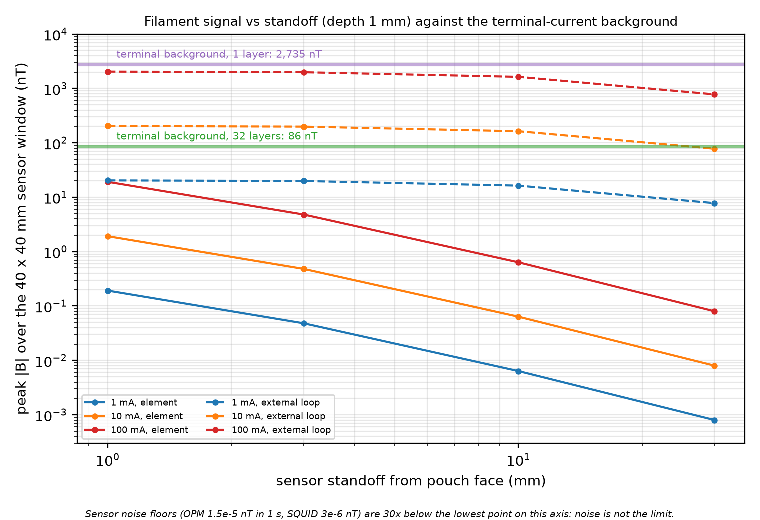
Filament signal against standoff for both return-path models; the 400× geometric spread dominates.

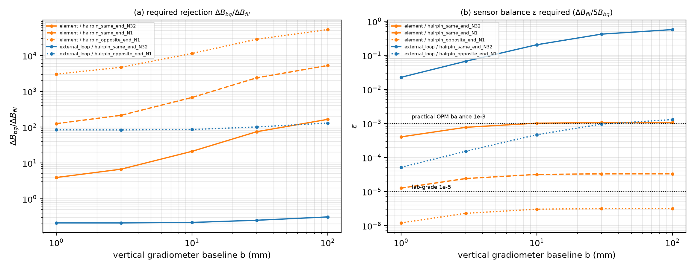
Gradiometer budget: required common-mode rejection against baseline; the optimum is b ≈ 1 mm.

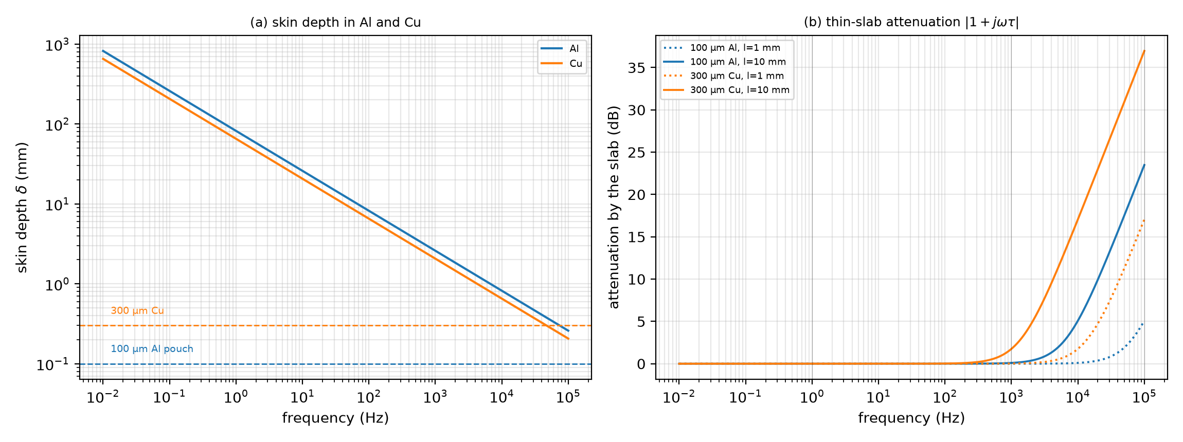
Eddy-current screening by the aluminium pouch and copper collector against frequency.

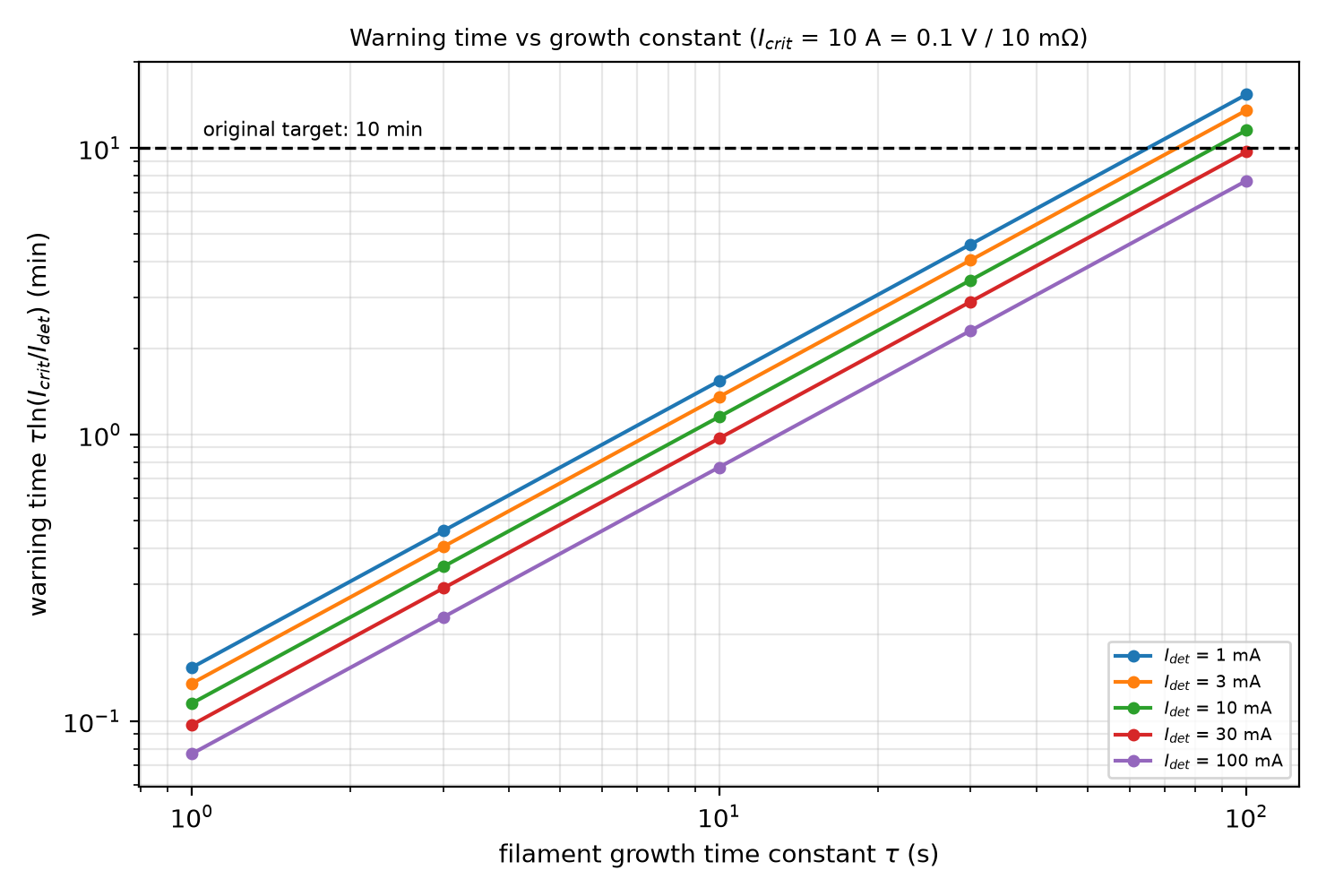
Warning time against the filament growth constant τ for each sensor class.

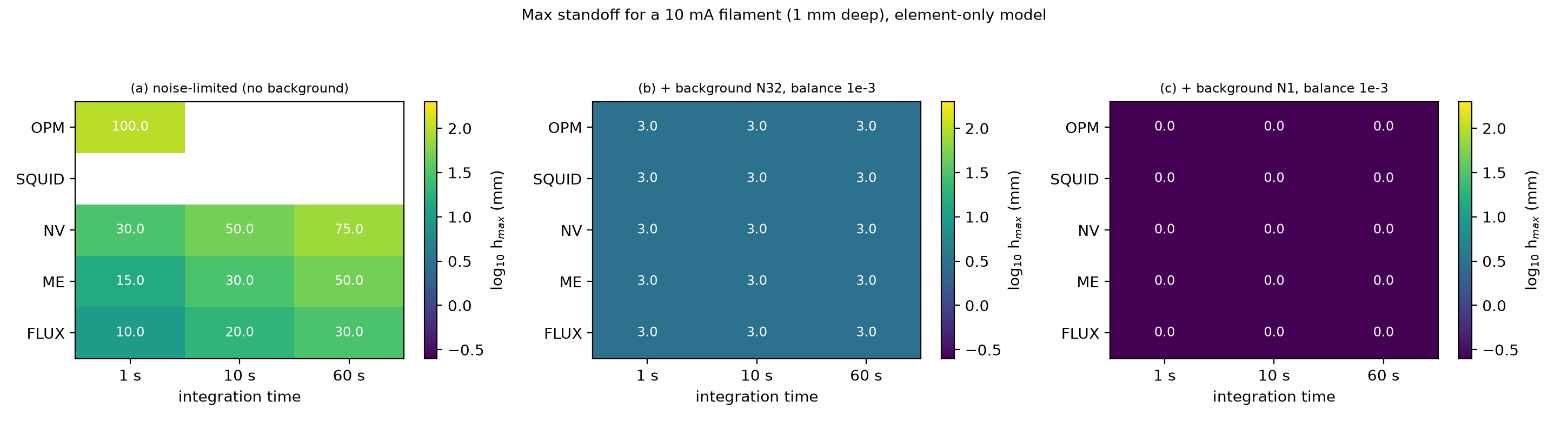
Decision table: maximum standoff per sensor class and background-rejection level.