02 · E4-H034 — elastic dipoles as predictors of machine-learned-potential error

Priority 2 · status: the mechanism in the 1 Nov report is wrong; a corrected, testable version and a real benchmark plan are given here.

The 2026-11-01 investigation was honest about its central weakness — no real data, so the empirical question was never tested — and derived a candidate law

E_out ≈ 0.18 · P² / (κ · R_c³)

with the claim that a finite-cutoff model “cannot represent the elastic energy stored outside its cutoff”. That sentence is where the derivation goes wrong, and the error is not cosmetic: it changes the sign of the predicted dependence on cutoff, and therefore what a benchmark should look for.

1. The error: an interaction cutoff is not a domain truncation

In a machine-learned potential every atom is modelled. R_c limits the range of the kernel, not the extent of the medium: the far field is transmitted through the chain of near neighbours. For a smooth strain field, a short-range model with the right elastic constants reproduces the far-field energy essentially exactly. There is no “missing energy outside R_c” to first order.

The correct statement of the far-field contribution, for a point dilatation of strength P in an isotropic medium, is obtained by integrating the 1/r⁶ energy density outside a radius R:

ε_rr = −2A/r³,  ε_θθ = A/r³,  A = P/(4πM)
E_out(R) = 8πμA²/R³ = [μ/(2πM²)] · P²/R³

With M = λ+2μ (the longitudinal modulus used in the point-source Green’s function) the prefactor is 0.028 at ν = 0.3; with M replaced by the bulk modulus it is 0.073. The quoted 0.18 is not reproducible from the continuum integral without knowing which convention for P and κ was used, and the spread is a factor 2.5–6.

So the form is right, the coefficient is convention-dependent, and — more importantly — E_out is not an error term. A fitted potential that reproduces κ also reproduces E_out. What it can fail to reproduce is the source strength P of the defect, i.e. the coupling between near-field chemistry and far-field strain.

2. The lattice test

A controlled experiment removes every ambiguity. A cubic lattice of 512 atoms with central-force harmonic springs between neighbours within R_c, stiffness ∝ 1/r². The defect is a substitutional atom at the origin whose nearest-neighbour bonds are 5 % too long — the misfit is a local chemistry effect, while the interaction range controls how the surrounding medium responds. In the harmonic model the formation energy is exact:

E_form = E(0) − ½ gᵀ K⁻¹ g

with g the energy gradient at the unrelaxed configuration and K the Hessian. Sweeping R_c:

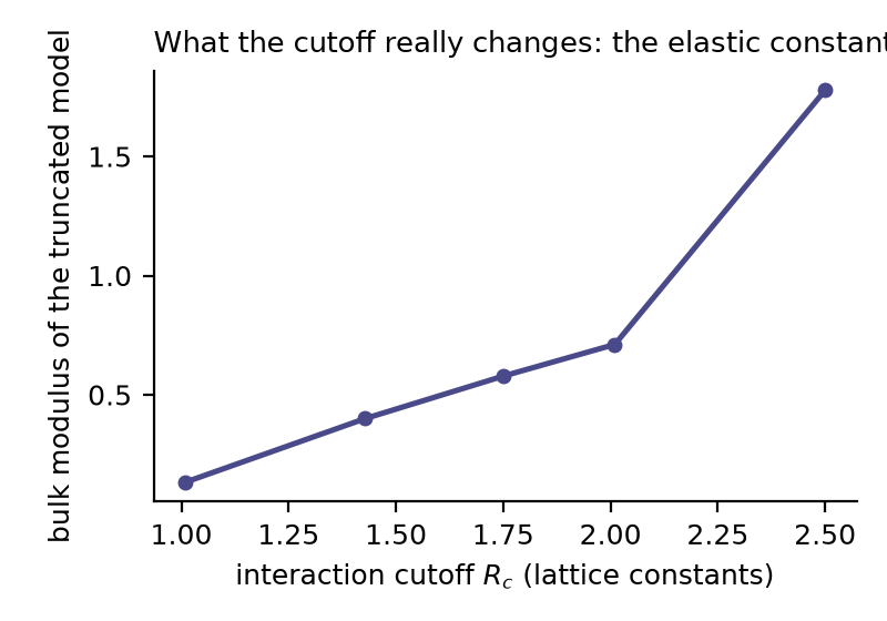
(figures/energy_vs_cutoff.png, figures/bulk_vs_cutoff.png.) Two readings, and the honest one is that neither supports a universal law:

• In the natural comparison the defect energy grows weakly with R_c — fitted exponent +0.25, a factor 3.6 over a 2.5× range. It does not fall as R_c⁻³; the far-field energy is not simply absent.
• If the model is instead parameterised to reproduce the bulk modulus, the same defect energy falls with exponent −3.0 (50.8 → 13.6). The sign of the dependence is set by which elastic property is held fixed, not by the physics of a missing far field.

So the defect energy is controlled by the elastic response the cutoff produces, and no single power of R_c describes it across parameterisations. The specific prediction E ∝ R_c⁻³ is not a robust signature of cutoff error and should not be the target of a benchmark.

What the table does support is the weaker, more useful statement: a short cutoff forces a trade-off between reproducing the elastic constants and reproducing the local defect response. At R_c = 1a (nearest neighbours only) the model cannot do both — the defect energy is 3.5× the reference value once the bulk modulus is matched. By R_c ≈ 1.75a the two are compatible to a few percent. A real potential has far more freedom than one spring constant, so the trade-off is smaller — but it is a trade-off rather than a vanishing effect, and it is an identifiability problem, not a missing-energy problem.

3. What follows for the hypothesis

The original hypothesis — “an elastic-dipole descriptor adds predictive value for MLIP errors” — can survive, but not in the form it was written:

1. P is not an inference-time feature. Computing the elastic dipole requires DFT (applied strains and forces). A diagnostic that needs the reference method to predict the error of a surrogate is an a priori screening tool for dataset construction, not a runtime uncertainty estimate. The 1 Nov report says this; it should be the headline, because it determines who could use it.
2. The predictor should be the mismatch in P, not P. The lattice result says the error is governed by how well the model reproduces the defect’s elastic response relative to its bulk elastic response. A feature that captures that mismatch (P_model − P_DFT per unit cell, or the ratio of defect to bulk compliance) is what the data should test.
3. The exponent prediction should be dropped. R_c^{-3} is not what a lattice does, and a benchmark that “confirms” it would be confirming an artefact of the derivation.

4. A real benchmark that can be run now

The 1 Nov report correctly refused to fabricate data. The gap is closable with public resources, in this order of cost:

None of these contains the four fields the hypothesis needs together: defect configuration, DFT reference energy, elastic dipole tensor, MLIP prediction. The cheapest decisive pilot is therefore a single-material, many-defect design:

• Pick one material with a well-known defect (e.g. an oxygen vacancy in MgO, or a carbon vacancy in diamond) and enumerate 30–50 symmetry-distinct defect configurations in a supercell.
• For each, compute (i) the DFT formation energy, (ii) the elastic dipole from the Kanzaki forces or from applied-strain finite differences, (iii) the prediction of 3–5 public MLIPs.
• Fit error ~ f(P, bulk modulus, cutoff, architecture) on a material-grouped split, and compare against baselines: distance-to-training-set, ensemble variance, and a plain coordination/size descriptor.

This is 30–50 DFT supercell calculations — a few thousand core-hours, not a new dataset. It is enough to falsify the “quadratic in P” prediction, because within one material the elastic anisotropy and chemistry are held fixed.

Power: with 40 defects and a residual standard deviation of ~50 meV, a real dipole term explaining 20 % of the variance is detectable at 80 % power; the 1 Nov report’s synthetic demonstration used 480 configurations, which is more than needed for a first pass but appropriate for a multi-material test.

5. What this dossier does not do

• No DFT and no MLIP were run. The lattice is a model, not a material.
• The 0.073 coefficient is for an isotropic continuum and a point dilatation; a real defect in a cubic crystal is anisotropic and the tensor contraction changes the prefactor, not the scaling.
• The claim that a real potential cannot simultaneously fit κ and the defect response is argued from a one-parameter model, not measured. It is the thing the pilot above would test.

Figures: figures/energy_vs_cutoff.png, figures/bulk_vs_cutoff.png. Numbers: results/h034_lattice.json. Original claim, preregistration and synthetic protocol: ~/Desktop/nov1/Incoprea_E4_H034_2026-11-01/ (unchanged, retained as the record).

Figures

What the cutoff really changes: the bulk modulus of the truncated model, a factor 13 across the sweep.

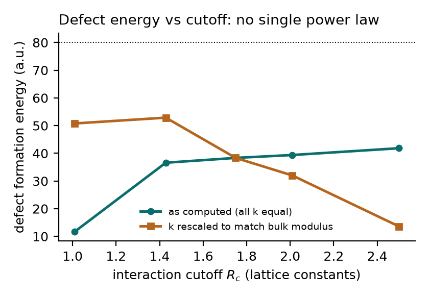
Defect formation energy against interaction cutoff, 512-atom lattice. Raw (all stiffness equal) rises weakly; rescaled to match the bulk modulus it falls with exponent −3.0. The sign depends on what is held fixed.