Priority 1 · status: published result reproduced, then substantially re-scoped.
The published test reports that reordering whole days inside each month raises the ideal cyclic storage capacity of a 70/30 wind/solar year by a median 10.7 % (updated to 10.9 %) across ten years of RTE data. This dossier reproduces that number to three significant figures, then asks the question the site itself lists as the next milestone: is the number a property of chronology, or of the null used to measure it?
Short answer: the arithmetic is right and the interpretation is not. The within-month day shuffle holds the multiset of days fixed but destroys multi-day persistence — real weather comes in runs, a shuffled year does not. When the null is made to preserve 3-day or 7-day runs, the premium collapses from 10.6 % to 5.1 % and 1.8 %. In a least-cost system with a firm fleet and a reliability target, the ordering effect is 1.3 % once persistence is preserved. The correct claim is narrower and more useful: storage sizing is sensitive to the run structure of the residual load, and the published number measures that sensitivity, not “chronology” as such.
| this dossier | published test | |
|---|---|---|
| median ratio (real year / within-month day-null) | 1.1083 | 1.1100 |
| years above their null | 10 / 10 | 10 / 10 |
| per-year ratio range | 1.033 – 1.271 | 1.027 – 1.271 |
| median ideal capacity | 31.6 TWh | 31.6 TWh |
| source rows | 175,344 | 175,344 |
Method: RTE éCO2mix national definitive half-hourly series,
2015–2024, wind and solar scaled so that wind carries 70 % and solar 30
% of annual demand; capacity = range of the cumulative net-load path (a
lossless cyclic store, no power limit, no efficiency). 999 permutations
of whole days within each calendar month. Code:
code/prepare_data.py, code/run_models.py
(model_A), figure
figures/capacity_by_year.png.
One data note worth recording: the “UTC” definitive file is
not on a clean UTC grid. On the ten spring-forward
dates the half-hour labels 01:00 and 01:30 UTC appear twice; on the ten
autumn dates 00:00 and 00:30 UTC are absent, which flags 30 calendar
days per decade. The row count still comes to exactly 175,344 because
the two errors cancel — a row-count check cannot catch this. Audit and
recomputation are in code/dst_audit.py /
results/dst_audit.json: dropping the 30 affected days moves
the median premium from 1.107 to
1.115, i.e. the defect is not material for a
day-level result, but it remains material for any sub-daily dispatch or
duration calculation, which must rebuild the timeline against the IANA
database first.
The null shuffles days, so every 2–10 day weather episode inside a
month is cut into independent days. Measured directly
(figures/runs.png): the longest run of worst-decile deficit
half-hours is 67 h in the real year (median over years)
and 38 h in the day-shuffle null. The null is not
exchangeable with the data it is meant to represent; it is a less
persistent system.
Replacing the null with a block shuffle — permute runs of L consecutive days inside each month, so L = 1 is the published null and L → month length approaches the real year — gives:
| block length L | 1 | 2 | 3 | 5 | 7 | 14 |
|---|---|---|---|---|---|---|
| median premium | +10.56 % | +7.59 % | +5.13 % | +3.24 % | +1.81 % | +1.48 % |
| years above null | 10/10 | 10/10 | 9/10 | 9/10 | 8/10 | 5/10 |
(figures/premium_vs_block.png.) The decline is monotone
and steep: three-quarters of the effect is gone once three-day runs are
preserved. It is not a subtle statistical quibble — it is the mechanism.
Capacity is the range of a cumulative sum, and the range is driven by
how long the system stays in deficit, not by which day sits before
which.
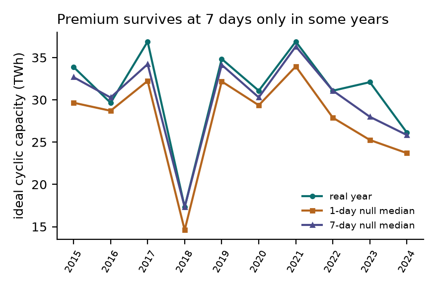
Two years still show a 7-day premium well above the rest (2023: +14.6 %, 2017: +7.8 %). Whatever distinguishes those years is the most interesting residual question here, and it is not answered in this dossier.
The ideal store has no power rating, no efficiency, no cost and no reliability target. Adding them:
Least-cost sizing. A stylised firm fleet (nuclear at
40 % of annual demand, hydro at 10 %, gas turbines at 15 % of peak)
leaves a residual that a battery and the gas fleet serve. Storage is
sized by minimising
100 k€/MW · P + 250 k€/MWh · E + 20 k€/MWh · unserved, 90 %
round-trip efficiency, perfect foresight, curtailment allowed, 11 null
draws per year. At that penalty the objective is dominated by unserved
energy (≈ 60 G€ of a 70 G€ total), so this ratio should be read as
“excess unserved energy”, not as a capital-cost premium — the
storage capex is under 1 % of the objective in every year.
| null | cost of the real year relative to the null median |
|---|---|
| 1-day shuffle (published null) | +16.3 % |
| 7-day block shuffle | +1.3 % |
Adequacy target. Same fleet, battery power fixed at 30 % of peak, battery energy sized so that unserved energy is ≤ 0.1 % of demand (a tight-standard proxy for LOLE):
| null | battery energy needed, real year relative to null median |
|---|---|
| 1-day shuffle | × 2.27 |
| 7-day block shuffle | × 1.27 |
(figures/cost_and_adequacy.png.) The second table is the
striking one, and it must be read with care: near a tight reliability
target the required energy is a knife-edge function of the worst run in
the year, so a factor of two is a statement about threshold sensitivity,
not about a stable “chronology cost”. The first table is the defensible
number: once the null preserves a week of weather, the ordering
of days is worth about 1 % of the modelled system objective — i.e. of
unserved energy — not 16 %.
The sign is also worth noting. With a firm fleet the battery’s value comes from short deficits; the real, run-heavy year needs less battery energy than a shuffled one (ratio of energies 0.47 at the 1-day null) while still costing more, because the runs exceed what any affordable battery can cover and the unserved energy is what costs money. Chronology does not simply “add storage” — it changes what storage is for.
At fixed peak, mean and variance, the within-month order of days changes the ideal cyclic storage capacity of a 70/30 wind/solar year by a median 10.6 %. Most of that number is the multi-day persistence that the day-shuffle null removes: preserving three-day runs halves it (5.1 %) and preserving seven-day runs reduces it to 1.8 %. In a least-cost system with firm capacity, the ordering effect is 1.3 % of cost under a persistence-preserving null. Sizing is therefore sensitive to run structure, and a day-shuffle null is not an adequate counterfactual for a weather-driven system.
This is compatible with the original proposal (which already included duration) and it does not rescue a universal “order matters” theorem. It does replace an unstable headline number with a mechanism that can be tested.
All numbers above are produced by code/run_models.py and
code/run_part2.py and stored in
results/summary.json and
results/summary_part2.json.
Ideal cyclic capacity by year: real, 1-day null median, 7-day null median. The premium survives at 7 days only in some years.
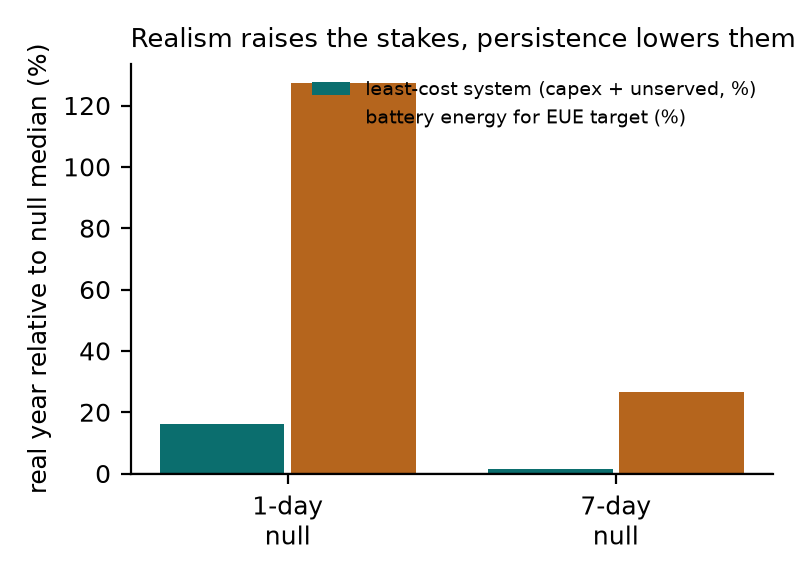
Least-cost system objective (dominated by unserved energy) and battery energy for a 0.1 % EUE target, under both nulls.
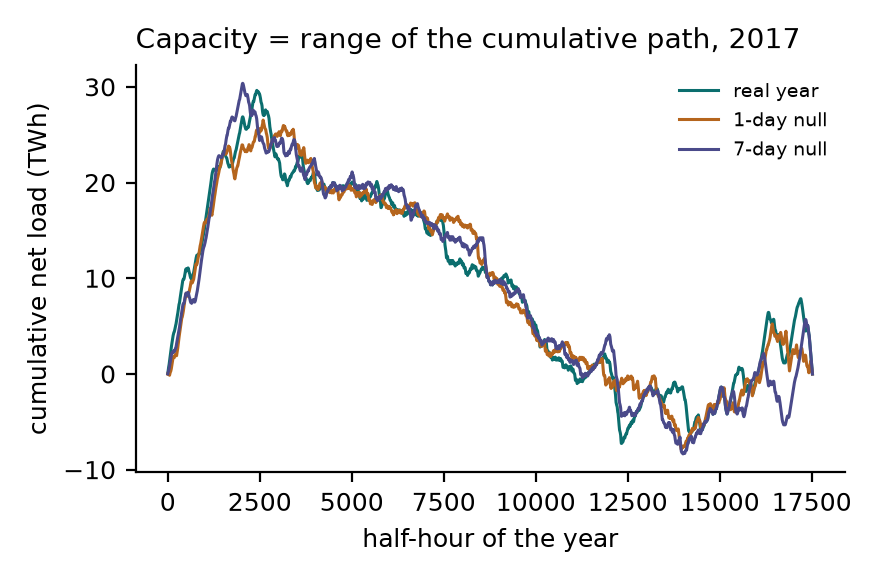
Cumulative net load for 2017. Ideal capacity is the range of this path; the three orderings differ in where the path turns, not in its endpoints.
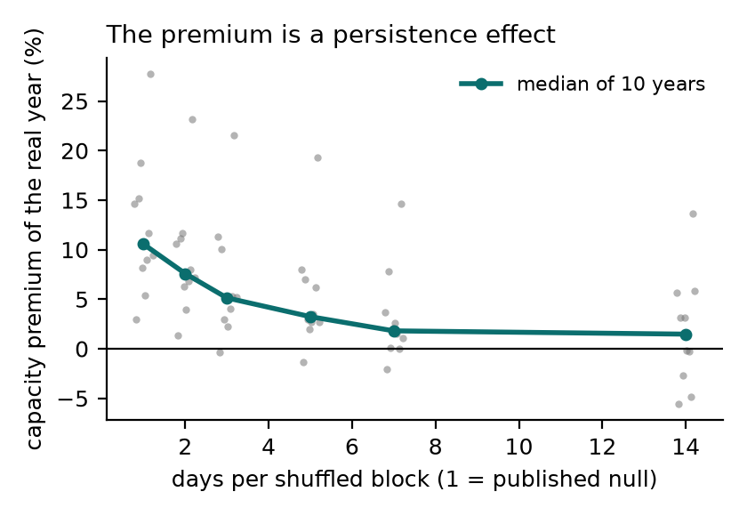
Capacity premium of the real year over a block-shuffled null, against block length. L = 1 is the published null. Grey dots are individual years; the line is the median.
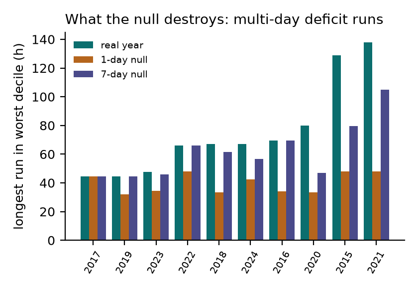
The longest run of worst-decile deficit half-hours, real year vs 1-day and 7-day nulls. This is what the day shuffle removes.